
Derive the Bias–Variance–Noise Decomposition for Squared Error
Retrain the same model on a different random split and the predictions move. Nobody changed the code. Nobody changed the hyperparameters. The wobble is not…

Key topics
Retrain the same model on a different random split and the predictions move. Nobody changed the code. Nobody changed the hyperparameters. The wobble is not a bug, and it is not noise in the data. It is a third thing, and the decomposition is the accounting that separates all three.
By the end of this article, you will be able to write the expectation, name every symbol, and prove the split yourself instead of reciting it.
Why One Error Number Hides Three Causes
A single test error conflates three distinct sources. A model that is systematically wrong. A model that is unstable across training sets. And randomness in the target itself that no model can remove.
The bias–variance decomposition is an accounting identity, not a new model. It does not predict anything on its own. What it does is tell you which cause you are actually paying for when your error is high.
If you have read the intuition-level treatment of the bias–variance tradeoff, you already have the diagnostic categories. Here we ask a sharper question: what do those words mean as exact mathematical objects? The shape of the result is:
Expected squared error = squared bias + variance + noise.
Each term has a different owner. Squared bias belongs to the model class and the fitting procedure. Variance belongs to the training data. Noise belongs to the data-generating process. Keep those owners in mind; they are the whole point.
Notation and the Data-Generating Assumptions
Before any algebra, fix the symbols. Every derivation mistake I have seen comes from losing track of what is random and what is fixed.
Fix a query point x. Define the target as
where is the true conditional mean, , and is noise with mean zero and variance . The noise is independent of the training set.
Define the learned predictor as . It is a random function because it depends on the random training set , drawn i.i.d. from the joint distribution .
Define the expectation over repeated draws of training sets, and the mean prediction:
The assumptions the derivation depends on:
- Squared loss.
- Additive noise with zero mean.
- Noise independent of the training data.
- A fixed query point .
Note: The noise term is irreducible only under these assumptions. Change them and the label becomes misleading, as we will see later.
One more distinction matters. In the fixed-design setting, the inputs are held fixed and all randomness comes from the noise . In the random-design setting, the inputs are also resampled. The fixed-design version tends to show larger bias and smaller variance, because less randomness lands in the variance term. Both are valid; they answer slightly different questions. I will use the random-design version because it matches how most people actually resample data.
Knowledge check
Check your understanding
Answer this question before you continue.
Deriving the Decomposition Step by Step
Start from the expected squared error at the fixed point :
The expectation runs over both the noise in and the randomness in the training set .
Step 1: Insert and subtract the mean prediction. Add and subtract inside the square:
Step 2: Expand the square. This gives three terms:
Step 3: Kill the cross term. This is the step most readers skip and most mistakes hide in. The factor has mean zero over , because is defined as the mean of . And it is independent of the noise in . So the expectation of the product factors into a product of expectations, and one factor is zero:
The cross term vanishes.
Step 4: Split the remaining two terms. The first term involves only and . Write :
The second term is the spread of predictions around their own mean:
Step 5: Write the identity.
In one plain sentence: average error = systematic miss + instability + unavoidable noise.
Knowledge check
Check your understanding
Answer this question before you continue.
A Small Worked Example You Can Check by Hand
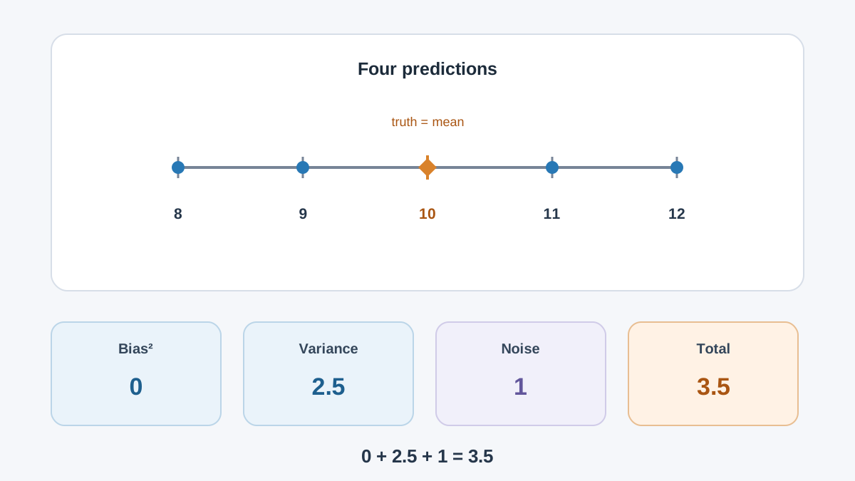
Abstract labels become real once you push numbers through them. Pick a query point where the true value is , and let the noise variance be .
Suppose your learner is a toy predictor whose output depends on which training set it saw. Enumerate four hypothetical training sets:
| Training set | Prediction |
|---|---|
| 8 | |
| 12 | |
| 9 | |
| 11 |
Mean prediction: .
Squared bias: .
Variance: the average squared deviation from the mean:
Noise: .
Total: .
Now verify directly. For each training set, the expected squared error at is the squared deviation from plus the noise variance:
- :
- :
- :
- :
Average: . The arithmetic closes. That closing is the proof.
Two sanity checks worth internalizing. Change the model and the noise term stays at 1. Change the true function and the variance term stays at 2.5. Each term answers to a different master.
If you want to verify this over many simulated training sets rather than four, the same arithmetic scales directly:
import numpy as np

rng = np.random.default_rng(0)
f_x = 10.0
sigma = 1.0
n_sets = 10_000

# Toy predictor: true value plus a training-set-dependent offset
offsets = rng.normal(0, np.sqrt(2.5), n_sets)
predictions = f_x + offsets

bias_sq = (f_x - predictions.mean()) ** 2
variance = predictions.var()
noise = sigma ** 2
print(bias_sq + variance + noise)
The printed value converges to roughly 3.5. The code confirms the hand calculation; it does not replace it.
Knowledge check
Check your understanding
Answer this question before you continue.
What Each Term Actually Owns
Squared bias is owned by the model class and the fitting procedure. It is the gap between the average prediction and the truth. The decomposition is evaluated for a specified learning procedure and a specified training-set size. Change either one and the bias term can move. A more flexible model class can reduce bias by representing more of the structure in ; a larger training set can also shift the expected fitted predictor, which is why "more data never helps bias" is too strong a claim.
Variance is owned by the learner's sensitivity to the particular training sample. It is the spread of predictions across resampled datasets. A model that memorizes its training set will have high variance: small changes in the data produce large changes in the fit.
Noise is owned by the data-generating process. No model, no amount of data, and no amount of tuning removes it under these assumptions.
The tradeoff is a statement about how a change in model flexibility moves two of the three terms in opposite directions. It is not a law that the sum must always improve. Sometimes adding flexibility cuts bias more than it adds variance; sometimes it does the reverse. The decomposition tells you which is happening; it does not tell you the answer in advance.
Common mistake: Assuming the clean three-way split transfers to classification. It does not. The decomposition is a squared-loss result. For 0-1 loss, cross-entropy, or classification accuracy, the terms do not simply add, and the "main prediction" is defined differently. Treat the decomposition as a reasoning tool for squared-error regression, and as a hypothesis generator elsewhere.
Knowledge check
Check your understanding
Answer this question before you continue.
From the Theorem to Training and Validation Curves
The theorem averages over infinitely many training sets. In practice you have one dataset, so you cannot compute directly. This is where most people confuse the idealized expectation with the quantities they can actually measure.
Training error and validation error are single-sample estimates. They are not bias and variance. A large train-validation gap is evidence about variance, not a measurement of it. The gap tells you the model fits its particular training sample much better than new data; it does not tell you how much of the gap is variance versus noise versus bias.
Resampling methods give you a practical proxy. Repeated splits, cross-validation, and bagging-style ensembles let you observe the spread of predictions across training sets. Averaging predictions over many resampled models is the closest practical analogue of . This is one reason ensembles can reduce the variance term: they approximate the mean prediction, and the mean prediction has no variance around itself. The size of that reduction depends on how the members are constructed and how correlated their errors are; averaging highly correlated models buys less than averaging diverse ones.
Common mistake: Reading a high validation error as proof of high bias. A high validation error does not tell you which term is large. You need a comparison across model complexity or across resamples to attribute the error. One number, one dataset, one model — that is not enough to separate the causes.
Assumptions That Break the Clean Split
The derivation is clean because the assumptions are strong. Here is where it stops being a reliable guide.
Nonzero-mean noise. If , the bias term absorbs the noise mean, and the "irreducible" label becomes misleading. The noise is still there; it is just hiding inside bias.
Residual dependence that breaks the cross-term argument. The cross term vanishes because the residual has mean zero at the fixed and is independent of the training-set randomness. What matters is that the held-out outcome's residual is mean-zero at and appropriately independent of the training procedure. A residual that is correlated with the input is not by itself a failure: as long as is the conditional mean, the residual can vary with and the pointwise decomposition still holds. The decomposition breaks when the residual's mean at is not zero, or when the training procedure and the held-out outcome are no longer independent in the way the cross-term argument requires.
Non-squared loss. Classification losses need different machinery. The decomposition changes form, and the terms do not simply add.
Distribution shift. If the data distribution changes between training and deployment, the expectation is taken over the wrong distribution. The decomposition describes a world that no longer exists.
The practical rule: use the decomposition as a reasoning tool for squared-error regression. Treat it as a hypothesis generator elsewhere, not a measurement.
Where to Go Next
Before you add complexity or collect more data, ask which of the three terms you are actually attacking. Then name the experiment that would show it.
A concrete next step: take a low-flexibility model and a high-flexibility model on your own regression data. Run both through repeated train-validation splits. Record the spread of predictions across resamples, not just the mean error. If the high-flexibility model's predictions swing widely across resamples while its average prediction barely moves, you are watching variance. To attribute bias, you need a known or defensibly estimated target function — as in a simulation or a controlled example where you set yourself. On ordinary data, the true conditional target is not directly observed, so a stable distance from one observed label cannot by itself identify bias. Repeated resampling tells you about prediction variability and model stability; bias attribution requires additional assumptions or comparisons.
That experiment turns the algebra into a debugging routine. The intuition-level tradeoff article gives you the diagnostic categories; the learning-curve article gives you the workflow. This derivation gives you the reason the categories are real.
Knowledge check
Final check
Finish the article by checking the ideas you just learned.
References
Build stronger machine learning foundations
Use structured resources to connect theory, scikit-learn workflows, and evaluation practice.


