
Derive the Cost-Sensitive Classification Threshold
A model returns 0.4. The default cutoff turns that into "negative," and nobody asked whether that was the right call.

Key topics
A model returns 0.4. The default cutoff turns that into "negative," and nobody asked whether that was the right call.
That single number — 0.5 — is doing more work than most people realize. It is not a neutral, fair, or scientific boundary. It is a cost assumption in disguise: the quiet claim that a false positive and a false negative hurt exactly the same amount. In fraud detection, medical screening, defect inspection, and content moderation, that claim is almost always false.
This article replaces the guess with a rule. We will derive the threshold that minimizes expected misclassification cost, work a small numerical example, and be honest about the assumptions the result depends on: calibrated probabilities, fixed per-error costs, and zero cost for correct predictions. If you already understand that a threshold converts scores into decisions and that moving it trades false positives against false negatives, you have everything you need to start.
Why 0.5 Is a Cost Assumption in Disguise
A classifier does not output decisions. It outputs scores, and a threshold converts those scores into labels. Move the threshold up and you get fewer positive predictions; move it down and you get more. That much is prerequisite intuition, and we will not re-teach it here.
What matters now is the hidden assumption inside the default. Predicting the positive class whenever is optimal only when both error types cost the same, correct predictions cost nothing, and the model is calibrated. Change any of those conditions and 0.5 stops being neutral — it becomes a silent policy choice that someone made by not making one.
Let's fix notation for the rest of the article:
- is the true label.
- is the predicted label.
- is the model's estimated probability that the example is positive.
- is the cost of predicting negative when the truth is positive — a false negative.
- is the cost of predicting positive when the truth is negative — a false positive.
Scope, stated up front: binary classification, costs that are fixed per error type and do not depend on the individual example, and probabilities that are already calibrated. If your probabilities are not calibrated, the threshold we derive is a precise number applied to the wrong quantity — and we will come back to that boundary.
Knowledge check
Check your understanding
Answer this question before you continue.
Set Up the Expected-Cost Objective
The derivation needs a target. That target is expected cost per example.
Assume correct predictions cost zero. That is a modeling choice, not a law of nature — it just means we only count the mistakes. With that assumption, each action has a clean expected cost:
- Predict positive. You are wrong only if the example is actually negative, which happens with probability $1 - p(x)(1 - p(x)) \cdot C(0, 1)$.
- Predict negative. You are wrong only if the example is actually positive, which happens with probability . Expected cost: .
Why is per-example expected cost the right objective? Because total expected cost over a dataset is the sum of per-example expected costs. Minimizing each term minimizes the sum. There is no global interaction to worry about — each decision stands alone.
Note: Costs that vary by example — a large transaction versus a small one — are a real and important case, but they need instance-dependent costs rather than a single threshold. That is out of scope here.
Knowledge check
Check your understanding
Answer this question before you continue.
Derive the Optimal Threshold Step by Step
Now the algebra. Predict positive whenever its expected cost is lower than the alternative:
Expand the left side:
Move the terms to one side:
Factor out :
Divide both sides by the positive quantity in parentheses:
That fraction is the threshold:
Read the symbols. The numerator is the cost of the mistake you make by predicting positive. The denominator is the total cost of both mistakes. The threshold is the share of total error cost that belongs to the false alarm.
The decision rule is now clean: predict positive when ; otherwise predict negative.
Sanity check. When , the threshold becomes . The default rule falls out as a special case. That is the whole point: 0.5 was never a law. It was the equal-cost case wearing a neutral mask.
Knowledge check
Check your understanding
Answer this question before you continue.
Work a Small Numerical Example
Suppose you are inspecting manufactured items. Missing a defect costs 10 units of pain — a returned product, a support ticket, a damaged reputation. Flagging a good item for manual review costs 1 unit — a few minutes of a human's time.
Operationally: flag anything above roughly 9% probability. Now watch what that does to individual scores.
| Score | Default 0.5 | Derived |
|---|---|---|
| 0.05 | negative | negative |
| 0.20 | negative | positive |
| 0.60 | positive | positive |
The 0.20 case is the interesting one. Under the default it slips through; under the derived threshold it gets caught. That is the cost asymmetry doing its job — you are deliberately buying recall with precision.
Now reverse the costs. Suppose a false negative costs 1 and a false positive costs 10 — say, an aggressive spam filter where wrongly blocking a legitimate email is far worse than letting spam through.
The threshold jumps to roughly 0.91. Now only very confident positives get flagged. The threshold moved in the opposite direction because the expensive mistake moved to the other side.
The general pattern: the threshold tracks the ratio of costs, not their absolute magnitude. Double both costs and does not budge.
Knowledge check
Check your understanding
Answer this question before you continue.
Read the Threshold as a Cost Ratio
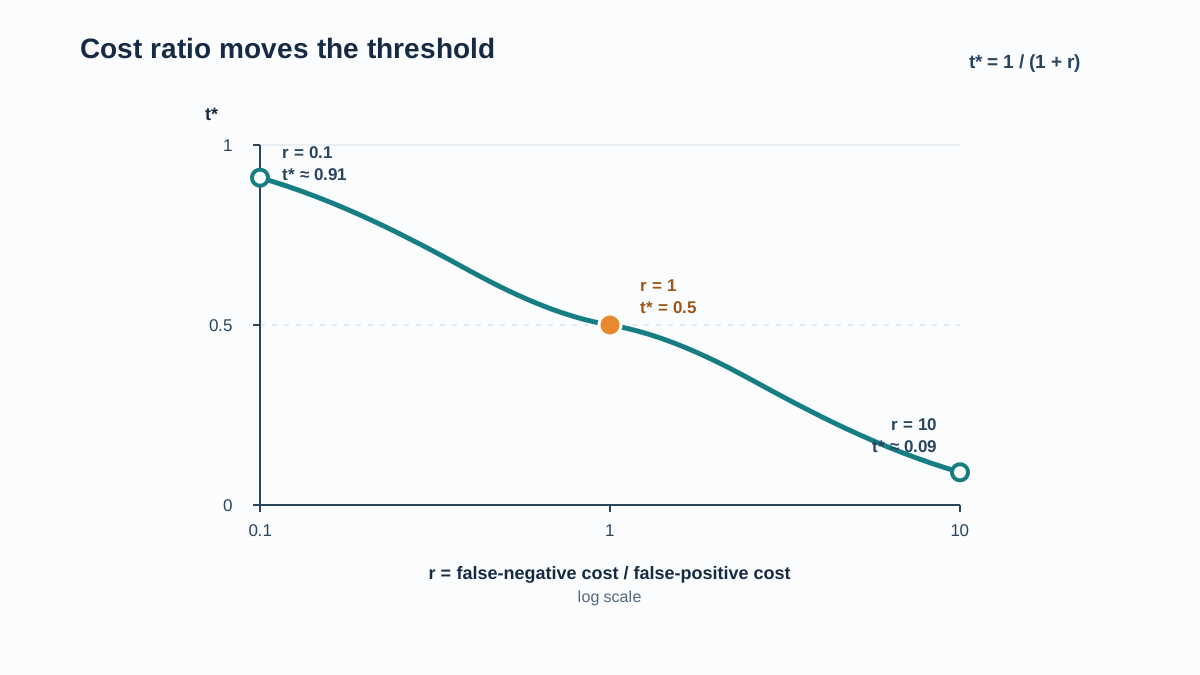
You do not want to re-derive this every time. Compress it into a mental model.
Let — the ratio of a missed positive to a false alarm. Then:
Now the direction is obvious. As missing positives gets relatively more expensive, grows and falls toward 0. As false alarms get relatively more expensive, shrinks and rises toward 1.
This is the Bayes decision threshold for binary classification, and it has a plain-English reading: a low threshold buys recall at the price of precision, and the cost ratio tells you how much precision you should be willing to spend. The threshold is where a cost judgment becomes a concrete operating point on the precision–recall tradeoff.
My rule: estimate the ratio first, then compute the threshold. Do not tune the threshold by feel and reverse-engineer the costs afterward. That path produces a magic number nobody can defend six months later.
When the Derivation Breaks Down
The formula is exact under its assumptions. The assumptions are where it gets fragile.
Calibration. If is not a calibrated probability — if a score of 0.2 does not actually mean a 20% chance — then is applied to a mis-scaled quantity. Check calibration before trusting the derived cutoff.
Fixed costs. Real costs often vary by example. A single threshold cannot express "this false negative costs more because the transaction is larger." That requires instance-dependent costs.
Costs are estimates. The formula is only as good as the numbers you feed it. In practice, small cost errors matter far less than getting the direction right — a 10:1 ratio and a 12:1 ratio produce similar thresholds.
Distribution shift. Here the two failure modes need separating. If the costs change — say, a missed defect now costs 50 instead of 10 — re-derive from the new numbers. If the population or prevalence changes, the cost-based threshold itself does not move; what moves is whether your probabilities still mean what they meant during training. A model calibrated on a 5% positive rate may be miscalibrated on a 20% positive rate, so the same now sits on top of unreliable scores. Check calibration on the new population before applying the old cutoff.
Practical fallback. When assumptions are shaky, tune the threshold empirically on validation data against a cost-weighted objective, and compare the result to the theoretical value as a sanity check. scikit-learn exposes threshold-tuning utilities for exactly this empirical comparison — the derivation here explains what those tools are approximating.
From Formula to a Working Decision Rule
Theory tells you why. Held-out data tells you whether you understood it.
Compute from your cost estimates, then verify it on data the model has not seen. Compare total cost at against the default 0.5 and against a small grid of nearby thresholds. If the empirical optimum sits far from the theoretical one, one of your assumptions is wrong — usually calibration or the cost estimates themselves.
Keep the cost assumptions written down next to the threshold. A threshold without its cost rationale is a magic number, and magic numbers rot.
Re-derive when costs change. Re-check calibration when the population shifts. Monitor the realized error mix in production rather than assuming the derivation still holds.
Here is your next step: pick one binary classifier you already have. Write down your false-positive and false-negative costs. Compute . Then compare its decisions to the default cutoff. The gap between those two sets of predictions is the cost of the assumption you were making without knowing it.
Knowledge check
Final check
Finish the article by checking the ideas you just learned.
References
Build stronger machine learning foundations
Use structured resources to connect theory, scikit-learn workflows, and evaluation practice.


