Run a K-Means Experiment: Inspect Clusters, Centers, and Scaling

Most people stop at fit(). They get a label array, scatter-plot it, and call the job done. But the label array is not the result — it is the beginning of the result. The real experiment starts when you read the centroids, change one input, and watch the partition move.

This is a reproducible drill: one dataset, one estimator, three deliberate perturbations. By the end, you will be able to print cluster labels, read centroid coordinates, and explain why a scaling change moved a point to a different cluster.

What This Experiment Will Prove

You already know the K-means loop: assign each point to the nearest centroid, recompute each centroid as the mean of its assigned points, repeat until stable. You also know that distance-based methods care about feature scale. This article does not re-teach either idea — it makes them visible in arrays you can inspect.

Here is what a finished experiment looks like:

• You can print cluster labels and read centroid coordinates.
• You can explain why a scaling change moved a point to a different cluster.
• You can compare partitions across different values of k without treating any of them as the "correct" answer.

Environment: Python with scikit-learn, NumPy, pandas, and matplotlib. No credentials, no external services, no downloads.

Dataset: A deterministic synthetic dataset via make_blobs with a fixed random_state, so every reader sees the same numbers.

import numpy as np
import pandas as pd
from sklearn.datasets import make_blobs

X, y_true = make_blobs(
    n_samples=300,
    centers=3,
    cluster_std=1.0,
    random_state=42,
)
df = pd.DataFrame(X, columns=["feature_a", "feature_b"])

We keep y_true aside. It is the ground truth from the generator, useful for sanity checks but not something you would have in a real clustering problem.

Fit K-Means and Read the Output

The smallest useful run:

from sklearn.cluster import KMeans

kmeans = KMeans(n_clusters=3, n_init=10, random_state=42)
kmeans.fit(df[["feature_a", "feature_b"]])

Two parameters control reproducibility. random_state fixes the seed for centroid initialization. n_init tells scikit-learn how many independent initializations to run; it keeps the best result by inertia. Set both, or your runs will differ between sessions.

Three fitted attributes matter:

Print them:

print("Label counts:", np.bincount(kmeans.labels_))
print("Centroids:\n", kmeans.cluster_centers_)
print("Inertia:", round(kmeans.inertia_, 2))

A healthy result looks like roughly balanced label counts and centroids that sit inside dense regions of the scatter. A collapsed result looks like one cluster holding almost every point and the others holding a handful — usually a sign of bad k, unscaled features, or duplicate points.

Why the code behaves this way: labels_ is the argmin of distance from each point to each centroid. cluster_centers_ is the mean of the points assigned to each cluster. The loop you already know is now visible as arrays.

Inspect Assignments and Centroids

Raw arrays are hard to reason about. Map the labels back onto the DataFrame so each row carries its cluster id:

df["cluster"] = kmeans.labels_
print(df.groupby("cluster")[["feature_a", "feature_b"]].mean())

That groupby mean should match cluster_centers_ — but only when the DataFrame rows are in the same order as the array you passed to fit(), and only when you compare the same feature columns in the same order. If you reordered rows, added columns, or fit on a subset, the comparison is invalid before it starts. Check those preconditions first; a genuine mismatch after that points to an indexing or fitting error.

Read centroids as feature-space averages, not as "typical members." A centroid can sit in a region with no data points at all, especially when a cluster is crescent-shaped or has an outlier pulling the mean sideways.

Check cluster sizes. Wildly unequal counts are a signal, not automatically a problem — but they deserve a look. If one cluster holds 280 of 300 points, ask whether the other two are real structure or noise the algorithm was forced to partition.

A scatter plot colored by label with centroids marked shows the Voronoi-style partition the algorithm produced:

import matplotlib.pyplot as plt

plt.scatter(df["feature_a"], df["feature_b"], c=df["cluster"], cmap="viridis", s=20)
plt.scatter(kmeans.cluster_centers_[:, 0], kmeans.cluster_centers_[:, 1],
            c="red", marker="x", s=200)
plt.show()

Experiment 1: Change the Scaling

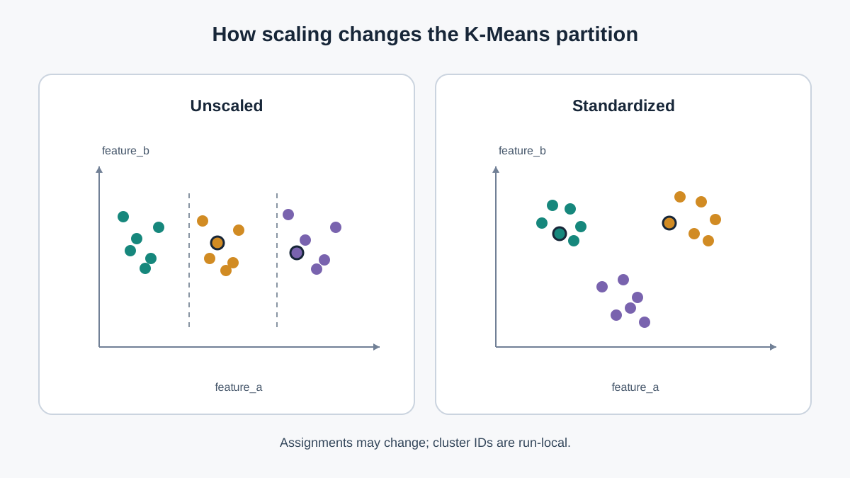
Now the first deliberate perturbation. Refit on unscaled features, then on StandardScaler-transformed features, and compare — but compare the right thing. Inertia is not comparable across these two runs, because scaling changes the units. What you can compare is which points changed cluster.

from sklearn.preprocessing import StandardScaler

scaler = StandardScaler()
X_scaled = scaler.fit_transform(df[["feature_a", "feature_b"]])

km_unscaled = KMeans(n_clusters=3, n_init=10, random_state=42).fit(df[["feature_a", "feature_b"]])
km_scaled   = KMeans(n_clusters=3, n_init=10, random_state=42).fit(X_scaled)

changed = km_unscaled.labels_ != km_scaled.labels_
print("Points that changed cluster:", changed.sum(), "of", len(changed))
print("Sample changed rows:\n", df[changed].head())

The mechanism: Euclidean distance sums squared differences across features. A feature with a large range contributes more to that sum, so it dominates the objective. Scaling puts every feature on comparable footing.

On this dataset, both features come from the same generator with the same spread, so scaling barely moves anything — you may see zero or only a handful of changed points. That is the honest result, and it is worth seeing. To force the effect, give one feature a much larger range and rerun:

df["feature_a"] = df["feature_a"] * 100
X_scaled = StandardScaler().fit_transform(df[["feature_a", "feature_b"]])
km_unscaled = KMeans(n_clusters=3, n_init=10, random_state=42).fit(df[["feature_a", "feature_b"]])
km_scaled   = KMeans(n_clusters=3, n_init=10, random_state=42).fit(X_scaled)
changed = km_unscaled.labels_ != km_scaled.labels_
print("Points that changed cluster after rescaling feature_a:", changed.sum())

Now the count jumps, and the sample rows show you exactly which points flipped. That is the observable signal the experiment is supposed to produce.

Common mistake: Comparing inertia between scaled and unscaled runs as if lower always means better clustering. Inertia is measured in the units of the feature space. When you scale, you change the units. The two numbers are not on the same ruler.

Experiment 2: Change the Number of Clusters

Second perturbation: loop over a small range of k, record inertia, and keep the fitted models so you can inspect membership later.

models = {}
inertias = []
for k in range(1, 9):
    km = KMeans(n_clusters=k, n_init=10, random_state=42).fit(X_scaled)
    models[k] = km
    inertias.append(km.inertia_)

plt.plot(range(1, 9), inertias, marker="o")
plt.xlabel("k")
plt.ylabel("inertia")
plt.show()

Inertia always decreases as k grows — more centroids can only reduce the within-cluster sum. The curve usually shows a bend where additional clusters stop buying much reduction. That bend is the elbow.

State the limit plainly: the elbow is a heuristic, not a verdict. A smooth curve means the data does not strongly favor one k. To see what adding clusters actually does, compare labels between two values of k:

labels_2 = models[2].labels_
labels_3 = models[3].labels_

# For each cluster at k=2, how many distinct k=3 clusters does it contain?
for c in np.unique(labels_2):
    members = labels_3[labels_2 == c]
    print(f"k=2 cluster {c} splits into k=3 clusters: {np.unique(members)}")

You will see that adding a cluster splits an existing group rather than discovering new structure. That is a useful observation, not a failure.

Judging whether any of these partitions is meaningful is a separate question, handled by stability tests and domain checks.

Failure Modes and Debugging Signals

When a K-means run goes wrong, the output usually tells you before the plot does.

• Convergence warnings. scikit-learn can warn that fewer distinct clusters were found than k. Usually duplicate or near-duplicate points, or a bad k.
• Empty or tiny clusters. Often a symptom of unscaled features or an over-large k.
• Outliers dragging centroids. A single extreme point can pull a center away from the dense region it should represent. Inspect the largest distances from each point to its centroid.
• Non-reproducible results. Forgetting random_state or setting n_init too low makes runs differ between sessions. If two runs disagree, you cannot tell whether the difference is real or initialization noise.

Make the Experiment Reproducible

Wrap the fit-and-inspect steps into a small function so you can point it at a new dataset instead of rewriting the inspection each time.

def kmeans_report(X, k, scale=False, random_state=42, n_init=10):
    from sklearn.preprocessing import StandardScaler
    if scale:
        X = StandardScaler().fit_transform(X)
    km = KMeans(n_clusters=k, n_init=n_init, random_state=random_state).fit(X)
    return {
        "labels": km.labels_,
        "centers": km.cluster_centers_,
        "inertia": km.inertia_,
        "k": k,
        "scaled": scale,
        "random_state": random_state,
        "n_init": n_init,
    }

Keep the scaling decision explicit as a parameter rather than a hidden default. Log random_state and n_init alongside the results so a run can be reproduced later. This is the reusable asset: a script you can point at a new dataset instead of rebuilding the inspection each time.

What to Carry Forward

Never report K-means output without stating three things: the scaling, the value of k, and the initialization settings. Those three choices produced the partition. Change any one of them and the labels change.

The next step is not to pick the "best" run. It is to test whether the clusters are stable and meaningful. Refit on bootstrap samples, check whether the same points stay together, and ask whether the groups correspond to something you can name. If they do not survive that scrutiny, the labels are a convenient partition, not discovered structure.