Derive the K-Means Objective and Its Assignment–Update Steps

Fit K-means twice on the same data with the same k, and you can get two different clusterings. The second run often reports a lower cost than the first. That single observation contains the whole theory: there is an objective, the algorithm only ever pushes it down, and the surface it descends has many valleys.

This article builds the formal spine. We will fix the notation, write the objective, derive both update steps as exact minimizers, and watch the objective fall in a hand-computed example. Then we will be precise about what convergence actually guarantees — and what it does not.

If you have already read the intuition piece on grouping data by proximity, treat scaling, choosing k, and interpreting clusters as given. Here we work on the objective itself.

What K-Means Is Actually Minimizing

Start with the data. We have $n$ points in $d$ dimensions, written as a matrix $X$ whose rows are the vectors $x_1, \dots, x_n$. The number of clusters $k$ is fixed in advance.

A clustering is a partition of the points into $k$ sets $C_1, \dots, C_k$. Disjoint, and covering every point: each point belongs to exactly one cluster.

The parameters the algorithm is allowed to move are the centroids $\mu_1, \dots, \mu_k$, each a vector in $\mathbb{R}^d$.

The K-means objective function — the within-cluster sum of squares, or WCSS — is:

$J = \sum_{j=1}^{k} \sum_{x_i \in C_j} \|x_i - \mu_j\|^2$

There is a second way to write the same quantity that makes the mechanism obvious:

$J = \sum_{i=1}^{n} \min_{1 \le j \le k} \|x_i - \mu_j\|^2$

Read that literally: every point pays for its distance to its nearest center, squared. The two forms are equal because each point's contribution depends only on the cluster it was assigned to, and the best assignment is always the nearest center.

Why squared Euclidean distance and not plain distance? Because the square is what makes the centroid update a closed-form mean. Swap in absolute distance and you get k-medians — a different objective with a different update rule. The choice of distance is the choice of algorithm.

Two Blocks, One Objective: Why the Problem Is Hard

Look at $J$ again. It depends on two coupled sets of unknowns: the partition and the centroids. You cannot optimize both at once in closed form.

But each one alone is easy. If the centroids were known, the best assignment is trivial — send each point to its nearest center. If the assignment were known, the best centroids are trivial — average the points in each cluster. Neither is known.

Brute force is not an option. The number of ways to partition $n$ points into $k$ groups grows on the scale of Stirling numbers, which explodes past toy sizes almost immediately.

So we use the standard strategy for coupled unknowns: hold one block fixed, minimize exactly over the other, repeat. This is alternating minimization, also called block coordinate descent. It is the same shape as the E and M steps in expectation-maximization.

One assumption to state plainly: $J$ is non-convex jointly. That fact is exactly why the guarantee we eventually prove is local, not global.

Deriving the Assignment Step

Hold the centroids $\mu_1, \dots, \mu_k$ fixed. Now $J$ becomes a sum of independent per-point terms, because each point's contribution depends only on which centroid it joins. No term couples two points.

For a single point $x_i$, its cost is $\|x_i - \mu_j\|^2$ for whichever $j$ it joins. Minimizing over $j$ means choosing the nearest centroid:

$C_j = \{ x_i : \|x_i - \mu_j\|^2 \le \|x_i - \mu_\ell\|^2 \text{ for all } \ell \}$

Squared distance and plain distance give the same argmin, so the square is harmless here — it only matters for the update step.

Geometrically, this step partitions space into Voronoi cells around the current centroids. Every point inside a cell is closer to that cell's center than to any other.

Note: When a point is equidistant from two centroids, the rule is ambiguous. Any consistent tie-break works; the objective value is unaffected. This is why two implementations can disagree on boundary points without either being wrong.

Why this step can only lower $J$: you are replacing each point's current cost with the minimum over all centroids, and a minimum is never larger than the value you started with.

Deriving the Centroid Update

Now hold the partition fixed. $J$ decomposes into $k$ independent subproblems, one per cluster, because no term couples two clusters. For cluster $C_j$, minimize:

$f(\mu) = \sum_{x_i \in C_j} \|x_i - \mu\|^2$

Take the gradient with respect to $\mu$. Each term contributes $2(\mu - x_i)$, so:

$\nabla f(\mu) = 2 \sum_{x_i \in C_j} (\mu - x_i) = 2 \left( |C_j| \mu - \sum_{x_i \in C_j} x_i \right)$

Set the gradient to zero:

$\mu_j = \frac{1}{|C_j|} \sum_{x_i \in C_j} x_i$

The mean falls out of the first-order condition. It is not a convention — it is the exact minimizer.

Check the second order: the Hessian is $2|C_j| I$, positive definite. This stationary point is a minimum, not a saddle or a maximum.

The interpretation is worth keeping: the mean is the point that minimizes total squared distance to a set of points. That is the entire justification for the update, and it is why the objective is defined with squares in the first place.

Warning: If a cluster receives no points, its mean is undefined. Real implementations handle this by reseeding or dropping the cluster. This is a genuine failure mode, not a footnote.

Lloyd's Algorithm as Alternating Minimization

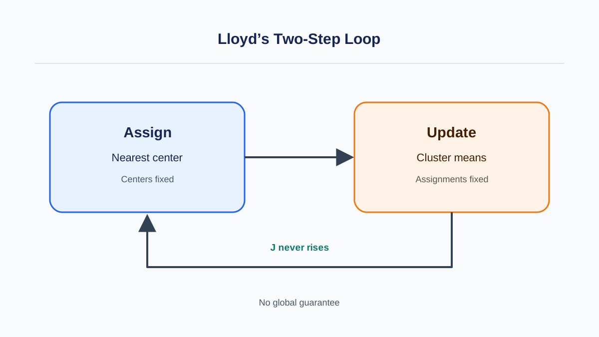
Assemble the two derived steps:

1. Initialize centroids $\mu_1, \dots, \mu_k$.
2. Assignment: assign each point to its nearest centroid.
3. Update: move each centroid to the mean of its assigned points.
4. Repeat until assignments stop changing, or centroid movement falls below a tolerance.

This is Lloyd's algorithm. Initialization is a required input, not part of the derivation. The objective says nothing about where to start — which is precisely why the starting point matters so much.

The standard seeding scheme is k-means++: pick the first center at random, then pick each subsequent center with probability weighted toward points far from existing centers. It does not change the objective. It changes which local minimum you tend to land in.

Convergence in practice is checked three ways — assignments unchanged, centroid shift below a threshold, or a maximum iteration cap. All three are stopping heuristics for the same underlying condition.

Cost per iteration is $O(n \cdot k \cdot d)$: every point is compared against every centroid. That is why K-means scales, and why $k$ and $d$ are the levers.

Worked Example: Watch the Objective Fall

Take six points on a line: $1, 2, 3, 10, 11, 12$. Let$k = 2$. Start with centroids at$\mu_1 = 1$and$\mu_2 = 12$.

Step 0 — initial objective. Assign by nearest centroid: $\{1,2,3\}$ to $\mu_1$, $\{10,11,12\}$ to $\mu_2$.

$J_0 = (0^2 + 1^2 + 2^2) + (2^2 + 1^2 + 0^2) = 5 + 5 = 10$

Step 1 — update. New means: $\mu_1 = (1+2+3)/3 = 2$, $\mu_2 = (10+11+12)/3 = 11$.

$J_1 = (1^2 + 0^2 + 1^2) + (1^2 + 0^2 + 1^2) = 2 + 2 = 4$

$J$ dropped from 10 to 4. The centroids moved to the true centers of their clusters.

Step 2 — assignment. Reassign by nearest centroid. Point 3 is distance 1 from $\mu_1 = 2$ and distance 8 from $\mu_2 = 11$ — stays. Point 10 is distance 8 from $\mu_1$ and 1 from $\mu_2$ — stays. No point changes cluster. The algorithm has stopped. Final $J = 4$.

Now rerun with a different initialization: $\mu_1 = 3$, $\mu_2 = 10$.

Assign: $\{1,2,3\}$ to $\mu_1$, $\{10,11,12\}$ to $\mu_2$. Update: $\mu_1 = 2$, $\mu_2 = 11$. Same answer. This dataset is too clean to trap the algorithm.

Make it harder. Start with $\mu_1 = 2$, $\mu_2 = 3$. Assign: point 1 goes to $\mu_1$, points 2 and 3 go to $\mu_2$, and points 10, 11, 12 go to $\mu_2$ as well. Now $\mu_1 = 1$ and $\mu_2 = (2+3+10+11+12)/5 = 7.6$.

$J = 0 + (5.6^2 + 4.6^2 + 2.4^2 + 3.4^2 + 4.4^2) \approx 104.8$

That is a local minimum the algorithm will settle into — and it is far worse than 4. Same data, same $k$, different answer. The objective tells you which one is worse.

A short scikit-learn check confirms the library minimizes exactly this quantity, exposed as inertia_:

import numpy as np
from sklearn.cluster import KMeans

X = np.array([[1], [2], [3], [10], [11], [12]])
km = KMeans(n_clusters=2, n_init=10, random_state=0).fit(X)
print(km.inertia_)          # within-cluster sum of squares
print(km.cluster_centers_)  # the means

The derivation is the point. The code is the receipt.

Why the Guarantee Stops at Local

Here is the convergence argument, stated precisely.

Each step weakly decreases $J$. The objective is bounded below by 0. And there are only finitely many distinct partitions of $n$ points into $k$ groups. A non-increasing sequence over a finite set must eventually repeat a state. Once a state repeats, the algorithm cycles — but since $J$ never increases, the cycle must be a fixed point.

What this proves: the algorithm terminates at a configuration where neither step can improve $J$. That is a local minimum of the alternating-minimization scheme.

What it does not prove: that no other partition achieves a lower $J$. The objective is non-convex, and the descent argument is blind to valleys the algorithm never visited.

The practical consequence is that results depend on initialization. Multiple restarts with different seeds, keeping the lowest final $J$, is the standard mitigation — and it is a mitigation, not a guarantee.

Common mistake: Reading "K-means converged" as "this is the best clustering." Those are different claims. Convergence means this run stopped improving, not this is optimal.

One theoretical footnote worth knowing: Lloyd's algorithm can require super-polynomial time on adversarial inputs, even in two dimensions. Typical inputs behave far better, so treat this as a known worst-case result rather than a practical warning.

What the Derivation Tells You to Do Next

The theory converts into four decision rules.

Always set a random seed and run multiple restarts. Compare final objective values, not just labels.

Scale features before fitting. The objective sums squared distances across dimensions, so an unscaled feature with large variance dominates the cost.

Treat a lower objective as a better fit to the stated cost — nothing more. The objective measures compactness under squared Euclidean distance. It does not measure whether the clusters mean anything.

When the objective plateaus across many values of $k$, that is a signal about the data's geometry, not proof of the right $k$.

The practical companion article runs this in scikit-learn and inspects assignments, centroids, and scaling effects. This article supplied the why; that one supplies the hands-on loop.

Before you move on, re-derive the centroid update from scratch on paper. Set up the sum of squared distances, take the gradient, set it to zero, and watch the mean appear. It takes two minutes, and it permanently converts the mean rule from a memorized fact into something you can reconstruct.