A Practical Clustering Workflow: From Unlabeled Data to Defensible Structure

Clustering always returns groups. Even on random noise, even on data with no structure worth naming, every algorithm will happily partition your points and hand you labels. That is not a bug—it is the job. The real skill is knowing which of those groups you can defend.

Here is the scene I see constantly: someone runs KMeans on a customer dataset, gets three clean-looking clusters, and announces they have discovered customer segments. The clusters exist. The segments probably do not. Between those two statements lies an entire unsupervised learning workflow—and skipping it is how beginners manufacture structure that was never there.

This article walks through that workflow as a chain of decisions: prepare data, choose a similarity metric, run multiple algorithms, validate without labels, use dimensionality reduction carefully, and interpret with discipline. Every link in the chain can create or destroy structure. Your job is to make sure the structure you report is the data's, not the algorithm's.

Why Clustering Output Is Not a Discovery

Clustering is an unsupervised learning method: it groups unlabeled data points so that points in the same group are more similar to each other than to points in other groups. That definition sounds like it is describing something the data contains. It is not. It is describing something the algorithm produces.

Run KMeans on purely random data and you will get clusters. Run it again with a different number of clusters and you will get different clusters. The algorithm does not know whether your data has real groups, and it does not care. It minimizes an objective function and returns a partition.

This is the central misconception that derails beginners: they treat algorithm output as discovered truth. But every clustering is a manufactured partition. Its defensibility depends entirely on choices made upstream—which features you kept, how you scaled them, which distance you used, which algorithm you ran, and how many clusters you asked for.

So the workflow is not "run clustering and see what you find." It is a chain of decisions where each link can manufacture or destroy structure. Get the chain right and you can make a claim like "these groups are stable and meaningful." Get it wrong and you have a partition that looks convincing and means nothing.

Prepare Data Before You Measure Similarity

Clustering algorithms group points by distance or similarity. That means your feature space literally defines what "similar" means. Change the features, change the scaling, and you change which points look close to each other.

The most common failure here is scale. K-means and hierarchical clustering both rely on distance geometry, and both silently let features with larger numeric ranges dominate the result. If one feature ranges from 0 to 1,000 and another from 0 to 1, the first feature will almost entirely determine which points cluster together. StandardScaler or MinMaxScaler fixes this by putting features on comparable footing—but only if you apply it before clustering, not after admiring your first confusing output.

Skewed features deserve attention too. A log transform on heavily skewed data can reveal structure that raw values hide, because extreme outliers stop compressing everyone else into one crowded region.

Mixed-type data is where preparation gets genuinely hard. One-hot encoding categorical features changes the geometry of your space in ways that are easy to underestimate. Text-like or high-dimensional sparse data often needs cosine distance rather than Euclidean. There is no universal answer here—only the discipline of asking what your distance metric will actually measure after you finish transforming the data.

Common mistake: Scaling the whole dataset before exploring it, then letting one wide-range feature decide your groups for you. Scale first, yes—but also look at your feature distributions and ask which ones deserve to influence similarity at all.

Choose a Similarity Metric That Matches Your Question

Similarity is not a property of your data. It is a judgment about what "alike" should mean for the question you are asking.

Euclidean distance is the default for good reason: it works well for dense, continuous features on the same scale, where magnitude matters. Two customers who spend similar amounts and visit with similar frequency land close together. That is often exactly what you want.

But Euclidean distance falls apart when magnitude should not dominate. Consider text documents or user-item interaction patterns. Two documents can share the same topics and themes while differing wildly in length. Cosine similarity measures the angle between vectors rather than their magnitude, so it captures directional similarity—"these documents are about the same things"—without punishing one for being longer.

My practical rule: pick the metric that makes two points you believe are alike actually land close together. Take a handful of examples you can reason about, compute their distances under a candidate metric, and sanity-check the ordering. If your metric says two obviously related points are far apart, the metric is wrong for your question—not the data.

Common mistake: Silently defaulting to Euclidean on mixed or high-dimensional data, then letting the metric decide your groups for you. The metric is a modeling choice. Make it deliberately.

Run More Than One Algorithm and Compare

Different clustering algorithms encode different definitions of what a cluster is. K-means finds convex, roughly equal-sized groups. DBSCAN finds density-based groups of arbitrary shape and flags outliers as noise. Hierarchical clustering reveals nested structure at multiple scales. None of these definitions is "correct"—each is a lens.

That is why running a single algorithm is weak evidence. If you run three algorithms with genuinely different assumptions and they land on similar groupings, that agreement is meaningful. It suggests the structure survives changes in method, which makes it more likely to be real rather than an artifact of one algorithm's quirks.

If the algorithms disagree, the disagreement is diagnostic. It tells you the structure is weak, the geometry is ambiguous, or your similarity choice is fighting your algorithm. All three are useful things to learn.

A practical pattern: run a fast method first to get a sense of the landscape, then confirm with a method that makes different assumptions. If KMeans suggests three groups, run DBSCAN and see whether density-based clusters tell a similar story. If they do not, you have learned something about your data before you ever interpret a single cluster.

Validate Structure Without a Ground Truth

Supervised learning has labels to check against. Unsupervised learning does not, and that makes validation inherently weaker. You are always assessing geometry, never meaning.

Internal validation metrics like the silhouette score measure how tight and well-separated your clusters are. They are useful—but they measure geometric properties, not semantic ones. A high silhouette score tells you the algorithm found compact, distinct groups under its own assumptions. It does not tell you those groups mean anything in the world.

Silhouette scores can also be fooled. Scale, outliers, and convex assumptions can inflate them. And here is the trap: if you tune the number of clusters to maximize silhouette, you are optimizing the algorithm's own objective and then treating the best-scoring partition as the "true" one. That is circular reasoning wearing a validation metric as a costume.

Common mistake: Tuning k to maximize silhouette and treating the best-scoring partition as ground truth. A high internal score is necessary but not sufficient evidence of meaningful groups. It confirms geometry, not meaning.

Use Dimensionality Reduction to See, Not to Prove

Principal component analysis is a powerful tool for compressing variation, denoising data, and making high-dimensional structure visible. It is not a validation method.

Running PCA before clustering can help: it discards low-variance noise and speeds up computation. But it also discards variance, and that discarded variance can contain exactly the signal that separates your groups. Projecting to two dimensions for a scatter plot is a visualization aid—nothing more.

Here is the uncomfortable truth about 2D projections: any high-dimensional structure can look like clusters or noise depending on the projection you choose. You can rotate a cloud of random points and find a view where they appear separated. Seeing separated blobs on a PCA scatter plot is not proof of real groups. The projection can create the illusion of separation.

Common mistake: Running PCA, seeing separated blobs on a 2D plot, and treating that as evidence of real structure. Use PCA to explore and communicate. Validate in the original feature space, or through agreement across algorithms.

Interpret Clusters and State What You Can Defend

Interpretation is where clustering turns into insight—or into overclaiming. The discipline is separating three levels of claim:

1. What the algorithm computed: "KMeans partitioned the data into four groups."
2. What the geometry shows: "The four groups are well-separated under Euclidean distance on these scaled features."
3. What you infer about the world: "These four groups represent distinct customer segments with different needs."

Only the third level needs domain justification. And it is the level where beginners routinely overreach.

Profiling each cluster is the first step: which features are high or low, what distinguishes one group from another, whether the profile matches domain sense. Check your clusters against known examples or external context when you have them. Agreement with prior knowledge strengthens your claim considerably.

Then resist the urge to name clusters with labels the data cannot support. If you measured purchase frequency and order size, you can say "frequent, high-spending customers." You cannot say "loyal customers who value premium quality"—that is a story you brought to the data, not one the data told you.

Common mistake: Naming clusters with causal or behavioral labels the data cannot support. If you cannot describe what makes each cluster distinct and why that distinction matters, you have a partition, not a finding.

The Decision Rule

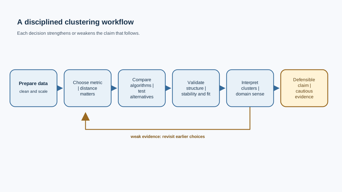
Run the chain: prepare, measure, compare, validate, interpret. Before you claim a meaningful group, ask whether the structure survives a different algorithm, a different metric, and a skeptical look at the projection.

Then try this as your next step: take a small, familiar dataset—something you already understand well—and run the full workflow. When you finish, write down in one sentence exactly what you can claim about the groups you found, and one sentence about what you cannot. That second sentence is where most clustering projects actually live. Learning to write it honestly is the difference between running an algorithm and doing unsupervised learning.

References

Research updated Sep 8, 2026