
Explore Hierarchical Clustering Linkages and Dendrogram Cuts
You fit the model, plot a tidy dendrogram, cut it at the biggest gap, and report three clusters. Then you change one argument — the linkage — and get a…

Key topics
You fit the model, plot a tidy dendrogram, cut it at the biggest gap, and report three clusters. Then you change one argument — the linkage — and get a different tree, a different gap, and a different count. Nothing about your data changed. Only the rule that decided which clusters were allowed to merge.
That is the whole lesson in one sentence: a dendrogram is a decision log, not a verdict. It records one greedy merge sequence under one distance rule. Change the rule and you get a different log.
This tutorial runs a compact experiment to make that concrete. One small dataset, four linkage rules, one scaling toggle, and a cut you can actually defend. By the end you will have a linkage matrix, four dendrograms, a table of cluster counts, and a clear sense of where the hierarchy stops being evidence.
What the Experiment Will Prove
The question is narrow on purpose: how much does the tree move when linkage, distance, and scaling change?
You need Python with scikit-learn, scipy, numpy, and matplotlib. No credentials, no external services, no downloads beyond the dataset that ships with scikit-learn.
I deliberately keep the sample small. Dendrogram inspection is most useful at small n, where you can still read individual leaves. At a few thousand rows the plot becomes a gray smear and you are back to trusting a number you cannot see.
Success criteria for this run:
- A linkage matrix
Zfrom SciPy. - Four dendrograms, one per linkage rule.
- A chosen cut height per linkage, derived from the largest gap in that linkage's merge distances.
- A table of cut heights, cluster counts, and sizes per configuration.
If you can produce that table and explain why the numbers differ, you have the skill this article is about.
Build the Linkage Matrix First
Here is the smallest useful step. We use a small mixed-scale dataset so scaling effects are visible later.
import numpy as np
from sklearn.datasets import load_iris
from sklearn.preprocessing import StandardScaler
from scipy.cluster.hierarchy import linkage, dendrogram, fcluster
import matplotlib.pyplot as plt

X = load_iris().data          # 150 rows, 4 features, different units
X_scaled = StandardScaler().fit_transform(X)

Z = linkage(X_scaled, method="ward")
print(Z.shape)                # (149, 4)
print(Z[-1])                  # final merge: member count == 150
A quick note on tooling: scikit-learn's AgglomerativeClustering fits labels directly, but it does not expose the full merge tree. For dendrogram work, SciPy is the tool. You will use both in this experiment — SciPy to build and inspect the tree, scikit-learn to fit flat clusters when you want them.
The linkage matrix has n - 1 rows. Each row is [cluster_a, cluster_b, merge_distance, member_count]. Three sanity checks before you plot anything:
- Row count equals
n_samples - 1. - The third column is non-decreasing — merges only get farther apart as you go up.
- The final row's member count equals
n_samples.
Common mistake: passing a precomputed distance matrix where a raw observation matrix is expected, or the reverse.
linkageaccepts either, and the two produce very different trees from identical-looking code. If your merge distances look like squared distances, check which form you passed.
Compare Linkage Rules on the Same Data
Now hold the data fixed and vary only the linkage method. Four rules matter most:
| Linkage | Merge rule | Typical shape |
|---|---|---|
| Single | Nearest pair of points | One long chain, a few large clusters |
| Complete | Farthest pair of points | Balanced, resists chaining |
| Average | Mean pairwise distance | Between the two above |
| Ward | Minimizes within-cluster variance increase | Compact, roughly equal-variance blobs |
The mechanism in one causal sentence each: single linkage chains through close neighbors, so a single bridge point can fuse two otherwise separate groups. Complete linkage resists that by measuring the worst-case gap. Average splits the difference. Ward does something different — it is not a distance between points but a variance criterion, and it prefers compact clusters of similar size.
methods = ["single", "complete", "average", "ward"]
fig, axes = plt.subplots(1, 4, figsize=(20, 5))

for ax, method in zip(axes, methods):
    Z = linkage(X_scaled, method=method)
    dendrogram(Z, ax=ax, truncate_mode="lastp", p=20)
    ax.set_title(method)
plt.tight_layout()
What to look for: single linkage usually produces one tall chain with a few late merges. Complete and average produce more balanced trees. Ward produces the most compact-looking splits on Euclidean data.
Warning: Ward is defined for Euclidean distance. Pairing it with cosine or Manhattan is a modeling error, not a tuning choice. Single, complete, and average accept a range of metrics; Ward does not.
Knowledge check
Check your understanding
Answer this question before you continue.
Read the Dendrogram Without Overreading It
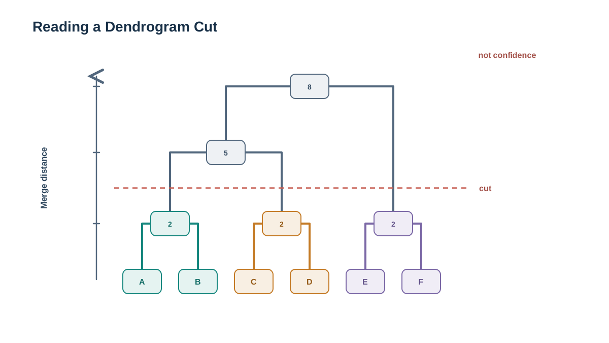
The visual grammar is simple once you stop projecting onto it.
Leaves are observations. Merge height is the distance at which two clusters joined. Branch length is that distance — not a probability, not a confidence, not a p-value.
The "biggest gap" heuristic is real but limited. A tall vertical jump suggests a natural cut because the algorithm had to travel far to make that merge. But the gap is a property of the merge sequence, not proof that the groups are separate in any meaningful sense.
Two things beginners consistently misread:
- Leaf order is not meaningful. The left-right order of branches can be flipped without changing the clustering. Do not read adjacency as similarity.
- Truncation hides detail, it does not remove it. With many leaves,
truncate_mode="lastp"andpkeep the plot legible. The hidden merges still happened.
The failure mode to watch for: a clean-looking tree that you treat as evidence of real groups, when the same data under another linkage produces a different clean-looking tree. Two clean pictures cannot both be the photograph.
Knowledge check
Check your understanding
Answer this question before you continue.
Cut the Tree and Check the Count
A cut turns the visual into a reproducible decision. There are two ways to do it:
- By number of clusters:
AgglomerativeClustering(n_clusters=k). - By distance threshold:
fcluster(Z, t=height, criterion="distance").
These are not interchangeable. A height cut can return a different count than you expected, and the same height means different things under different linkages because the distance scales differ.
To make the cut reproducible, derive it from the largest gap in each linkage's own merge distances. The largest gap is the biggest jump between consecutive merge heights — the point where the algorithm had to travel farthest to combine the next pair of clusters.
def largest_gap_height(Z):
    heights = Z[:, 2]
    gaps = np.diff(heights)
    return heights[np.argmax(gaps) + 1]

for method in methods:
    Z = linkage(X_scaled, method=method)
    height = largest_gap_height(Z)
    labels = fcluster(Z, t=height, criterion="distance")
    counts = np.bincount(labels)[1:]
    print(f"{method:9s} height={height:.2f} clusters={len(counts)} sizes={sorted(counts, reverse=True)}")
The output is the table the success criteria promised: one cut height, one cluster count, and one size distribution per linkage. The heights will not match across linkages — they are measured on different distance scales. That is the point. A single fixed height applied to all four linkages would be an arbitrary choice dressed up as a rule.
Uneven sizes are a signal, not automatically a problem — but a single dominant cluster plus a few tiny ones usually means the cut is too high.
Connect this to validation: a cut is a hypothesis about structure. Stability across linkages is weak evidence in its favor. Instability is strong evidence against a single confident claim.
Knowledge check
Check your understanding
Answer this question before you continue.
Scaling Changes the Tree, Not Just the Numbers
Hierarchical clustering is distance-based. A feature measured in large units dominates the merge order unless features are standardized. That is not a numerical detail — it reshapes the hierarchy.
Run the same linkage on unscaled and standardized data:
Z_raw = linkage(X, method="ward")
Z_scaled = linkage(X_scaled, method="ward")
print("raw max merge:", Z_raw[-1, 2])
print("scaled max merge:", Z_scaled[-1, 2])
The merge heights, the gap location, and the cluster membership all shift. On the iris data, the raw version is largely a petal-length tree because that feature has the widest numeric range.
Standardization is not automatically correct. If your units are meaningful and comparable — say, all features are already in the same currency or the same physical scale — scaling can erase real signal. The decision rule is whether the units are commensurable, not whether scaling is "best practice."
Tip: If one feature's variance dwarfs the others, the tree is mostly that feature's tree. Check the variance ratio before you trust the shape.
Knowledge check
Check your understanding
Answer this question before you continue.
Where the Hierarchy Stops Being Evidence
A dendrogram is a deterministic record of greedy merges under one distance and one linkage rule. It is not a statistical test of group existence.
Three limits worth naming plainly:
- Greedy merges are irreversible. An early bad merge propagates upward and cannot be undone later. The tree carries its own history.
- There is no inherent cluster count. The algorithm always produces a full tree, even on data with no group structure at all. A dendrogram of pure noise still looks like a dendrogram.
- Branch height is not significance. It is a distance under your chosen metric. It says nothing about whether the split corresponds to a real-world category.
What would strengthen a claim: stability across linkages and resampling, agreement with domain knowledge, and separation that survives scaling changes. What should not be assumed: that cluster labels are ordered or meaningful, or that a visually separated branch maps to a real category.
One Modification Worth Trying
The most useful follow-up is a stability check. Rerun the whole pipeline on bootstrap resamples and record how often each pair of observations lands in the same cluster — normalized by how often that pair was actually sampled together.
rng = np.random.default_rng(0)
n = X_scaled.shape[0]
co_cluster = np.zeros((n, n))
co_sampled = np.zeros((n, n))

for _ in range(50):
    idx = rng.integers(0, n, n)
    Zb = linkage(X_scaled[idx], method="ward")
    labels = fcluster(Zb, t=largest_gap_height(Zb), criterion="distance")
    for i in range(n):
        for j in range(i + 1, n):
            a, b = idx[i], idx[j]
            co_sampled[a, b] += 1
            co_sampled[b, a] += 1
            if labels[i] == labels[j]:
                co_cluster[a, b] += 1
                co_cluster[b, a] += 1

with np.errstate(invalid="ignore", divide="ignore"):
    stability = np.where(co_sampled > 0, co_cluster / co_sampled, np.nan)
Now stability[i, j] is a frequency between 0 and 1: the fraction of resamples where both observations were present and landed in the same cluster. Pairs near 1 support a stable structure. Pairs near 0.5 flip depending on the sample. Pairs near 0 were rarely together.
Without the co_sampled normalization, a pair that happened to appear in more resamples would look more stable simply because it had more chances to co-cluster. The frequency removes that bias.
A second variation: swap Euclidean for Manhattan or cosine distance with single, complete, or average linkage. Ward is no longer valid in that swap — remember why.
Keep the scope small. The goal is to see the tree move, not to build a production pipeline.
If your chosen cut does not survive a modest perturbation, report the structure as exploratory rather than established.
The Habit That Makes This Stick
Never report a hierarchical clustering result without naming four things: the linkage, the distance metric, the scaling decision, and the cut rule. Those four choices produced the tree. Without them, the tree is not reproducible and not interpretable.
I have watched this trip up experienced engineers who would never report a regression without its features. Clustering gets a pass because the output looks like a picture. It is not a picture. It is a log.
Your next step: take a dataset you already care about, run the four-linkage comparison, and see which cut survives a bootstrap. If none of them do, you have learned something more valuable than a cluster count — you have learned that the structure is not there yet.
Knowledge check
Final check
Finish the article by checking the ideas you just learned.
References
Build stronger machine learning foundations
Use structured resources to connect theory, scikit-learn workflows, and evaluation practice.


