Test Clustering Stability Across Resamples and Settings

Your clusters looked clean until you changed the random seed. Now the labels shuffled, the boundaries moved, and you are not sure whether you found structure or just a lucky draw. A clustering stability experiment answers that question directly: perturb the data or the algorithm, compare the assignments, and see whether the partition survives.

Stability is not proof that your groups mean something. It is proof that they reproduce. That distinction is the whole game.

What Stability Actually Measures

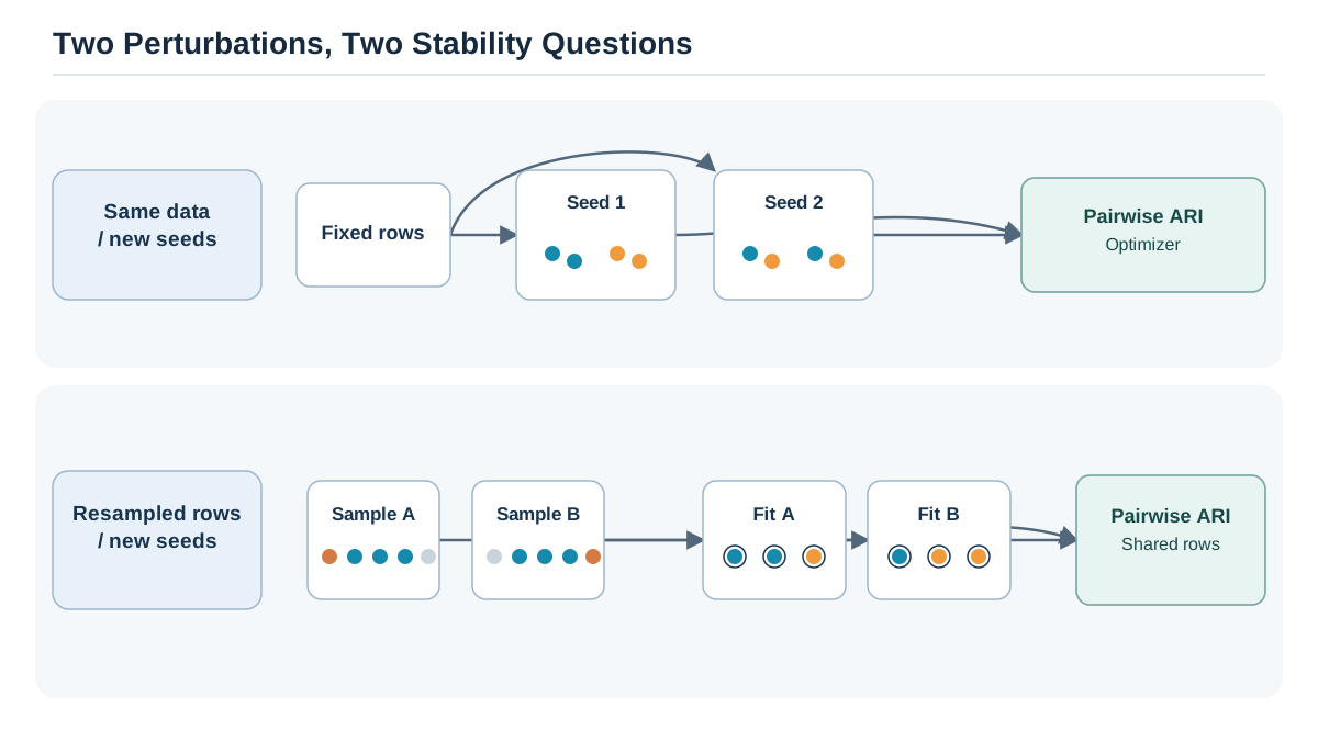
Stability measures how much cluster assignments agree when you perturb either the data or the algorithm. If a partition is stable, small changes to the input or the starting conditions produce roughly the same grouping. If it is unstable, the grouping was an artifact of one particular run.

There are two perturbation families, and they answer different questions:

• Resampling (bootstrap or subsample) asks: does the structure depend on which rows happened to be in the dataset? You draw new samples, cluster each one, and compare assignments on the points they share.
• Initialization (multiple random starts) asks: does the optimizer land in the same place every time? You fit the same algorithm on the same data with different seeds and compare the results.

These can disagree, and the disagreement is informative. A solution that is stable across seeds but unstable across resamples is sensitive to which rows you collected. A solution that is stable across resamples but unstable across seeds is sensitive to the optimizer, not the data.

Here is the boundary you must hold onto: stability is about reproducibility of the partition, not about whether the partition is meaningful. A single dense blob split into three parts can be perfectly stable and still be three arbitrary slices of one thing. Stability tells you the answer is reproducible. It does not tell you the answer is right.

This is why stability complements internal metrics like silhouette score rather than replacing them. Silhouette measures geometry: are points close to their own cluster and far from others? Stability measures persistence: does the partition hold up when you disturb the inputs? You want both, and you want domain interpretation on top.

If your assignments are unstable, every downstream decision built on them—naming a segment, targeting a group, writing a report—is built on sand. That is the practical stake.

Set Up a Bounded Experiment

You need Python with scikit-learn, NumPy, and pandas. No external services, no credentials. Keep the experiment small enough to inspect.

Pick one dataset and one algorithm. I will use K-means on a scaled feature matrix, but the harness works for GMM or agglomerative clustering with minor changes. The critical rule: fix your preprocessing pipeline first and reuse it identically across every run. If you scale one run and not the next, you are comparing two different datasets, not two clusterings.

Define the perturbation grid before you run anything. For initialization, 10–20 random seeds. For resampling, 20–50 bootstrap draws. State your success criterion up front: what agreement level would make you trust the assignment, and what would make you suspicious?

import numpy as np
from sklearn.cluster import KMeans
from sklearn.preprocessing import StandardScaler
from sklearn.metrics import adjusted_rand_score

rng = np.random.RandomState(0)

# Three well-separated blobs plus a little noise, so we know the truth.
centers = np.array([[0, 0, 0, 0], [6, 6, 6, 6], [-6, 6, -6, 6]], dtype=float)
X = np.vstack([c + rng.normal(scale=0.8, size=(100, 4)) for c in centers])

scaler = StandardScaler().fit(X)
Xs = scaler.transform(X)  # same scaled data for every run

def fit_labels(data, seed, k=3):
    km = KMeans(n_clusters=k, n_init=1, random_state=seed)
    return km.fit_predict(data)

The n_init=1 matters here. By default, scikit-learn runs K-means several times internally and keeps the best result, which hides the initialization sensitivity you are trying to measure. Set it to 1 so each seed produces exactly one answer.

The synthetic data gives you a known answer: three blobs, three clusters. That is the point. You are testing whether the harness can recover a structure you already trust before you point it at data where you do not know the truth.

Compare Assignments With Adjusted Rand Index

You need one summary statistic that compares two labelings of the same points. That statistic is the adjusted Rand index (ARI).

ARI has two properties that make it the right tool:

1. It is invariant to label permutation. Cluster 0 in run A can match cluster 2 in run B. ARI does not care about the names, only about which points are grouped together.
2. It is adjusted for chance. Random labelings score near 0 in expectation. This is exactly what you need when comparing many runs, because it gives you a meaningful baseline.

Raw Rand index and raw mutual information do not have the second property. They drift upward as the number of clusters grows, so a finer-grained labeling looks more "agreeable" even when it is random. That makes them useless as a consensus index. Only chance-adjusted measures can be safely used to evaluate average stability across overlapping subsamples.

Reading scale:

ARI value	Interpretation
Near 1.0	Assignments essentially identical
Around 0.5	Moderate agreement, some points move
Near 0.0	No better than chance
Negative	Worse than chance

Report the distribution, not a single number. One lucky pair of runs proves nothing. You want the mean, the spread, and the low tail.

Run the Resampling and Initialization Variants

Now turn the scaffold into two concrete experiments.

Initialization variant. Fit the same algorithm on the same data with different seeds, then compute pairwise ARI across all runs.

seeds = range(10)
labels_by_seed = [fit_labels(Xs, s) for s in seeds]

ari_init = [
    adjusted_rand_score(labels_by_seed[i], labels_by_seed[j])
    for i in range(len(seeds))
    for j in range(i + 1, len(seeds))
]
print(f"init ARI mean={np.mean(ari_init):.3f} min={np.min(ari_init):.3f}")

On the three-blob data, this prints something like init ARI mean=1.000 min=1.000. Every seed recovers the same partition. That is what a stable solution looks like when the structure is unambiguous.

Resampling variant. Fit on bootstrap draws, then compare assignments on the overlapping points.

n = Xs.shape[0]
n_boot = 30
boot_labels = []
for b in range(n_boot):
    idx = rng.choice(n, size=n, replace=True)
    lab = fit_labels(Xs[idx], seed=b)
    boot_labels.append((idx, lab))

ari_boot = []
for i in range(n_boot):
    for j in range(i + 1, n_boot):
        idx_i, lab_i = boot_labels[i]
        idx_j, lab_j = boot_labels[j]
        common = np.intersect1d(idx_i, idx_j)
        if len(common) < 10:
            continue
        map_i = dict(zip(idx_i, lab_i))
        map_j = dict(zip(idx_j, lab_j))
        a_i = np.array([map_i[c] for c in common])
        a_j = np.array([map_j[c] for c in common])
        ari_boot.append(adjusted_rand_score(a_i, a_j))
print(f"boot ARI mean={np.mean(ari_boot):.3f} min={np.min(ari_boot):.3f}")

Here you should see boot ARI mean=1.000 min=1.000 as well, or very close to it. The blobs are far enough apart that dropping rows does not move the boundaries. That is the success criterion: a clean structure should survive both perturbations.

The np.intersect1d step is not optional. When you compare across subsamples, you must only compare points present in both runs. Scoring ARI on different row sets produces a meaningless number. If you would rather keep all points, project held-out points onto the fitted centroids before scoring instead.

Interpret the two variants separately. They can disagree, and that disagreement tells you which kind of fragility you have.

Read the Results Without Overclaiming

High stability is necessary but not sufficient. Low stability is strong evidence against a claim.

The sober finding from the literature is worth internalizing: stability does not reliably identify the "correct" number of clusters, and for large samples it can be uninformative about validity. Treat it as a reproducibility check, not a model-selection oracle. A stable clustering of noise is still noise.

Watch for degenerate cases. Clusters of very different sizes, or a k that is too large, can inflate or deflate agreement in ways that have nothing to do with real structure. When k is too large, the algorithm randomly splits true clusters, and which cluster it splits changes with the sample—so instability can be a symptom of over-splitting rather than of weak structure.

My decision rule: stable + supported by an internal metric + interpretable in domain terms = worth investigating further. Stable alone = not enough.

Failure Modes and Debugging Signals

Most stability experiments go wrong in predictable ways. Here is the checklist.

• Scaling changed between runs. The most common silent bug. Verify the preprocessing object is identical across every fit. If you refit the scaler on each bootstrap sample, you have introduced a second source of variation you did not intend to measure.
• Comparing labels without aligning points. Scoring ARI on different row sets produces garbage. Always intersect first.
• Too few resamples. Three runs cannot distinguish a stable solution from a lucky one. Use enough draws to see a distribution.
• Interpreting a high ARI as proof of truth. It is proof of reproducibility, nothing more.
• Ignoring the low tail. A mean ARI of 0.8 with occasional runs at 0.2 tells a very different story than a tight 0.8. The tail is where the fragility lives.

Common mistake: Refitting the scaler inside the resampling loop. It feels natural—each sample gets its own preprocessing—but it changes the comparison. Fit the scaler once on the full dataset and reuse it.

One Follow-Up Experiment

Stability becomes a habit when you build it into a reusable harness. Here are three extensions that turn the drill into a system.

Sweep k. Run the same harness across a small range of cluster counts and plot mean ARI against k. Look for a plateau rather than a single peak. A sharp peak is often noise; a broad plateau suggests a range of reasonable solutions.

Swap the algorithm. Rerun the same harness with GMM or agglomerative clustering. This is a sensitivity check on your modeling assumptions, not a validity test. Different algorithms impose different notions of cluster shape, so they can disagree even when real structure exists. When they do agree, that is useful supporting evidence. When they do not, you have learned that your conclusion depends on the geometry you assumed—which is worth knowing before you act on it.

Add a noise control. Run the entire experiment on shuffled or synthetic random data. If your real data scores no better than the control, you have your answer. This is the cheapest sanity check in the whole workflow, and it is the one people skip.

Keep the harness as a function so future clustering work gets the same check for free. The next time you fit a model and the plot looks tidy, you will have a number that tells you whether to trust it—or a number that tells you to rewrite the question.

Stable assignments earn the right to be investigated. Unstable ones earn a rewrite. Combine this stability check with internal validation metrics and domain interpretation before you name a single cluster.