
Experiment With DBSCAN in Scikit-Learn: Parameters, Scaling, and Noise
Change one number in a DBSCAN call and the whole story of your data can flip: two clusters become one, or a clean grouping dissolves into a field of noise.…

Key topics
Change one number in a DBSCAN call and the whole story of your data can flip: two clusters become one, or a clean grouping dissolves into a field of noise. Same data, same algorithm, different answer. That sensitivity is not a bug — it is the mechanism, and the fastest way to understand it is to hold the data fixed and move one knob at a time.
This is a controlled experiment. We will build a small, reproducible setup, inspect the raw labels before trusting any plot, sweep eps and min_samples, compare scaled against unscaled inputs, and treat cluster scores as diagnostics rather than verdicts. If you already know what core, border, and noise points mean, you have everything you need to start.
Set Up a Reproducible DBSCAN Experiment
You need Python with scikit-learn, NumPy, and matplotlib. No external services, no credentials, no data downloads. We generate the data ourselves so we always know the ground-truth shape.
import numpy as np
from sklearn.datasets import make_moons
from sklearn.cluster import DBSCAN
from sklearn.preprocessing import StandardScaler

X, y_true = make_moons(n_samples=300, noise=0.06, random_state=42)
make_moons gives us two interleaving crescents. That shape matters: it is exactly the kind of non-convex structure where centroid-based methods struggle and density-based methods should shine. If DBSCAN cannot find two crescents here, that is a diagnostic signal — either the parameters are off, or the geometry is not what you assumed. Investigate before concluding the data is at fault.
Now a small helper so every run is comparable:
def run_dbscan(X, eps, min_samples):
    labels = DBSCAN(eps=eps, min_samples=min_samples).fit_predict(X)
    n_clusters = len(set(labels)) - (1 if -1 in labels else 0)
    n_noise = np.sum(labels == -1)
    return labels, n_clusters, n_noise
Two disciplines keep this honest. First, we reuse the same X array in every run — no regenerating data between comparisons. Second, DBSCAN is deterministic given fixed input, so unlike K-means there is no random_state to worry about inside the algorithm itself. Any difference you see comes from a parameter or from the data's geometry, never from initialization luck.
Read the Labels Before You Trust the Plot
Before plotting anything, look at the raw output. A scatter plot is persuasive; the label array is honest.
labels, n_clusters, n_noise = run_dbscan(X, eps=0.3, min_samples=5)
print("clusters:", n_clusters, "noise:", n_noise)
print("unique labels:", np.unique(labels))
labels_ returns cluster ids starting at 0, with -1 reserved for noise. That -1 is a label, not a missing value — it is the algorithm telling you "this point did not belong to any dense region." Counting clusters means excluding -1 from the unique set. Forget that step and you inflate your cluster count by one every time noise exists.
There is a second distinction hiding in the output. core_sample_indices_ tells you which points are core points — the ones with enough neighbors to seed and expand a cluster. Border points belong to a cluster but cannot grow it. When you plot, coloring core and border points differently often explains why a cluster has the shape it does.
Common mistake: A tidy two-dimensional scatter can look convincing even when the structure is an artifact of the parameters. The numbers — cluster count and noise count — are your first check, not the picture.
Knowledge check
Check your understanding
Answer this question before you continue.
Sweep eps and Watch Clusters Merge and Dissolve
eps sets the neighborhood radius. It defines what counts as "close enough" to be density-connected. It is not a maximum distance within a cluster — chains of neighborhoods can span far more than eps. That distinction is the whole reason DBSCAN finds curved shapes.
Let's sweep it:
for eps in [0.1, 0.2, 0.3, 0.5, 0.8]:
    _, n_clusters, n_noise = run_dbscan(X, eps=eps, min_samples=5)
    print(f"eps={eps:<4} clusters={n_clusters:<3} noise={n_noise}")
The trend is legible at a glance:
| eps | clusters | noise |
|---|---|---|
| 0.1 | many | high |
| 0.2 | ~2 | moderate |
| 0.3 | ~2 | low |
| 0.5 | 1 | near 0 |
| 0.8 | 1 | 0 |
Treat this table as qualitative tendencies, not exact output. Your printed numbers are the success criterion — read them, not the table. Small eps fragments dense regions into many tiny clusters and pushes most points into noise; the radius is too short to connect neighbors. Large eps merges genuinely separate groups into one blob and collapses the noise count toward zero. The useful range lives between those failures.
A practical starting heuristic is the k-distance graph: for each point, plot the distance to its k-th nearest neighbor (with k roughly equal to min_samples), sort the distances, and look for the "knee" where the curve bends upward. That bend is a reasonable first guess for eps. It is a heuristic, not a derivation — treat it as a starting point, then sweep around it.
Knowledge check
Check your understanding
Answer this question before you continue.
Sweep min_samples and See What Counts as Dense
min_samples is the density threshold: how many neighbors a point needs before it can seed a cluster. It does not act independently of eps — the two are coupled.
for min_samples in [2, 3, 5, 10, 20]:
    _, n_clusters, n_noise = run_dbscan(X, eps=0.3, min_samples=min_samples)
    print(f"min_samples={min_samples:<3} clusters={n_clusters:<3} noise={n_noise}")
Raising min_samples demands more neighbors before a point can seed a cluster, so sparse regions become noise. Lowering it toward 1 turns DBSCAN into something closer to single-linkage behavior, where almost nothing is noise and clusters chain together. Watch a single run: bump min_samples from 5 to 20 with eps fixed, and points that were clustered migrate into the noise bucket. The mechanism is direct — the density bar rose, and those points no longer clear it.
A common rule of thumb is min_samples >= dimensions + 1, with small values like 3 to 5 as a reasonable start for low-dimensional data. The coupling matters more than the exact number: a larger eps with a larger min_samples can produce results similar to a smaller eps with a smaller min_samples. Sweep them together, not one at a time in isolation.
Knowledge check
Check your understanding
Answer this question before you continue.
Compare Scaled and Unscaled Inputs
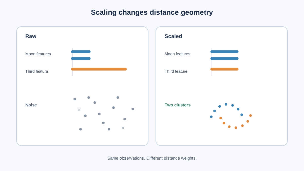
DBSCAN uses Euclidean distance by default. That means a feature measured in the thousands dominates one measured in single digits — not because it is more important, but because it is numerically larger. Scaling does not change the algorithm; it changes the geometry the algorithm sees.
To make the failure mode visible, we need a deliberate scale mismatch. make_moons alone will not show it: both coordinates already share a similar range, so scaling barely moves the result. Add a third feature on a much larger scale and the picture changes.
rng = np.random.default_rng(0)
third_feature = rng.normal(loc=500.0, scale=50.0, size=(X.shape[0], 1))
X_wide = np.hstack([X, third_feature])

X_wide_scaled = StandardScaler().fit_transform(X_wide)

for name, data in [("raw", X_wide), ("scaled", X_wide_scaled)]:
    _, n_clusters, n_noise = run_dbscan(data, eps=0.3, min_samples=5)
    print(f"{name:<7} clusters={n_clusters:<3} noise={n_noise}")
On the raw X_wide, the third feature sits around 500 with a spread of about 50. Its contribution to squared Euclidean distance dwarfs the crescents' coordinates, which live roughly between -1 and 2. The crescents effectively disappear: the distance metric is now measuring the third feature, and the moons become a smear. After standardization, all three features contribute on comparable terms, and the crescent structure returns.
That is the whole lesson. Scaling is not cosmetic; it decides which feature the distance metric actually listens to.
After scaling, eps is expressed in the units of the standardized space. It is a radius in the full multivariate distance, not a separate per-feature cutoff. A value like 0.3 means "points within 0.3 units of each other in the scaled feature space," where each unit is roughly one standard deviation of a feature. That is more interpretable than an arbitrary raw number, but it is still a joint distance across all features — not a threshold applied to each one independently.
Warning: If this experiment is a step inside a larger supervised workflow, fit the scaler on training data only. Fitting on the full dataset leaks information from your test set into preprocessing.
One boundary worth remembering: distance-based methods like DBSCAN and K-means both care about scale. Tree-based models do not, because they split on thresholds rather than distances. When you switch between these families, the scaling requirement switches with them.
Knowledge check
Check your understanding
Answer this question before you continue.
Use Cluster Scores as Diagnostics, Not Verdicts
It is tempting to compute a silhouette score and treat a high number as proof the clusters are real. Resist that.
Silhouette and similar internal metrics assume roughly convex, well-separated groups — precisely the assumption DBSCAN is designed to relax. Applying a convexity-loving metric to a density-based result measures the wrong thing. Worse, noise points labeled -1 must be handled deliberately before computing any score, or the metric silently includes them as if they were a cluster.
A score can improve while the clustering becomes less useful for your actual question. The metric is a diagnostic, not a decision. What is often more informative is stability: if clusters survive a range of eps values, that is weak evidence of real structure. If the cluster count swings wildly between adjacent parameter settings, you are probably looking at an artifact.
For the full treatment of internal metrics, stability tests, and domain validation, the clustering validation material is the right next step. Here, just remember: a clean plot and a good score are inputs to judgment, not substitutes for it.
Debug the Runs That Go Wrong
Most DBSCAN failures fall into a few recognizable patterns:
- Everything is noise.
epsis too small for the current scale, or features are unscaled and one dimension dominates the distance. - One giant cluster.
epsis too large, ormin_samplesis too low, so density chains connect everything. - Cluster count changes wildly between runs. The data may not have density structure at all, or the parameters sit on a knife edge.
- Results differ from a tutorial you copied. Check whether that tutorial scaled its features and you did not.
- Memory blowup on large data. scikit-learn's implementation can degrade toward quadratic memory when
epsis large andmin_samplesis low.
Each of these is a signal about the geometry, not a reason to abandon the method. Read the signal, adjust one variable, and re-run.
Run One More Experiment Yourself
The point of this article is not the code you copied — it is the mechanism you now control. Prove it to yourself with one modification.
Take the X_wide array from the scaling section and try a non-Euclidean metric such as metric='manhattan' or metric='cosine'. Notice how the meaning of eps shifts with the metric — the same number now measures a different kind of distance, and the cluster and noise counts change accordingly. Then re-run the scaled version with the same metric and compare.
If you want a sharper contrast, run K-means on the same scaled data and compare. K-means will cut the crescents into two roughly circular blobs; DBSCAN will trace their curves. That difference is the geometric assumption made visible.
Record your parameter grid and the resulting cluster and noise counts in a small table. Reproducibility is not ceremony — it is how you turn a one-time result into evidence you can defend later.
The parameters are a lens, not a setting. eps and min_samples decide what the algorithm is allowed to see; scaling decides what the data looks like before the algorithm looks at it. My rule: scale first, sweep eps and min_samples together, and inspect the noise count before you trust any score. When you are ready to judge whether the groups you found are worth acting on, the clustering validation material is where that judgment gets built.
Knowledge check
Final check
Finish the article by checking the ideas you just learned.
References
Build stronger machine learning foundations
Use structured resources to connect theory, scikit-learn workflows, and evaluation practice.


