Gradient Boosting Explained: How Small Corrections Become a Strong Model

Random forests grow many trees independently and average their votes. Gradient boosting grows trees one at a time, each one aimed at the mistakes the current model still makes. That single difference changes how you train, tune, and think about the model.

The mental shift: from averaging trees to correcting them

If you have worked with random forests, you already know the bagging story: grow many deep trees on random samples of the data, let each one vote, and average away the noise. The forest works because individual trees are noisy, but their errors are only weakly correlated, so the average is steadier than any single tree.

Gradient boosting is a different bet. Instead of spreading effort evenly across the data, it keeps pushing where the model is still wrong.

Think of a forest as a committee that votes. A boosted model is more like a sculptor: each new tree is another pass that removes material where the shape is still off. The committee spreads its attention; the sculptor concentrates on what remains broken.

This is the core distinction between bagging and boosting. Bagging mainly reduces variance by averaging. Boosting mainly reduces bias by sequential correction. A forest asks many independent models what they think and combines their answers. A boosted model asks each new learner one question: what did the current model get wrong?

What each new tree actually learns

Let us make this concrete with a regression example, because the mechanism is easiest to see when the target is a number.

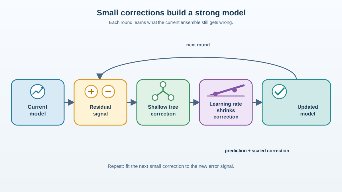
Suppose you are predicting house prices. Your first tree looks at the data and makes its best guesses. Some predictions are too high, some too low. For each house, you can compute the residual: the true price minus the predicted price. A positive residual means the model under-predicted; a negative one means it over-predicted.

Now here is the move that defines gradient boosting: you train the second tree not on the original prices, but on those residuals. The second tree learns to predict the error the first tree made.

When you add the second tree's prediction to the first tree's prediction, the combined model is more accurate wherever the first tree was off. Then you compute new residuals against the combined model and train a third tree on those. Then a fourth. Then a fifth.

The final prediction is an additive model:

final prediction = first prediction + correction 1 + correction 2 + ...

Each new tree is a correction term, not a full model on its own. A single shallow tree in the middle of a boosted ensemble is almost meaningless in isolation. Its job is only to nudge the overall prediction in the right direction for the cases the current ensemble still gets wrong.

Watch what happens to the residuals as corrections stack up. The first tree might leave large errors scattered across the data. The second tree removes part of those errors. The third tree targets what remains. With each step, the residuals shrink, and the model's predictions creep closer to the true values.

This is why boosting can beat bagging on many problems. A random forest spends equal effort on every region of the data. Boosting spends extra effort exactly where the model is still failing.

Why it is called gradient boosting

The residual story is intuitive, but it only works directly for squared-error loss. What if you are doing classification, or ranking, or any other prediction task where "subtract prediction from truth" does not make sense?

This is where the word gradient enters.

For squared-error loss, the residual turns out to be proportional to the negative gradient of the loss with respect to the prediction. In plain language: the residual points in the direction the prediction should move to reduce error. If the model under-predicts, the residual is positive, and the prediction needs to move up. If it over-predicts, the residual is negative, and the prediction needs to move down.

Gradient boosting generalizes this idea. For any loss function you care about, you can compute the gradient of that loss with respect to the current predictions. That gradient tells you, for each training example, which direction the prediction should shift to increase the loss. To reduce the loss, you move the opposite way—the negative gradient. So instead of fitting each new tree to a plain residual, you fit it to this negative-gradient direction, often called the pseudo-residual.

That is the whole trick. The machinery stays the same whether you are doing regression with squared error, classification with log loss, or something more exotic. You swap the loss function, compute the negative gradient, fit a tree to it, and add the correction. The name gradient boosting is just a reminder that each tree points the model downhill on error.

One clarification matters for classification. A boosted classifier does not literally train each new tree on a column of 0/1 mistakes. It works with a loss function and the model's current prediction scores, so the next tree targets the loss's local correction signal. "Mistakes" is a useful intuition, not the literal training target in every task.

You do not need to do calculus by hand to use gradient boosting. Libraries handle the gradients for you. But understanding where the name comes from helps you see why the method is so general: it is not a special algorithm for residuals. It is a general recipe for minimizing any differentiable loss by sequential correction.

The learning rate: how big each correction should be

If each new tree added its full correction, the model would lurch toward the training data and overshoot. Gradient boosting prevents this with a shrinkage factor called the learning rate.

The learning rate scales down every correction before it is added. A learning rate of 0.1 means each new tree only contributes one-tenth of its raw prediction to the ensemble. The remaining nine-tenths are not wasted—they are simply not applied in this step. Later trees can continue refining the same direction.

Why take such small steps? Because small corrections are more careful than big ones. A large correction might fix the current error but overshoot into a new one. A small correction moves the model gently in the right direction, and the next tree can refine the adjustment.

This creates a direct tradeoff between the learning rate and the number of trees. With a small learning rate, each tree contributes less, so you need more trees to reach the same accuracy. With a large learning rate, each tree contributes more, so you need fewer trees, but the risk of overshooting and overfitting rises.

The practical pairing is simple: lower the learning rate, and you usually need to raise the number of estimators to compensate. A common beginner mistake is to crank up the number of trees while keeping a large learning rate, then wonder why the model overfits. The two dials move together.

Common mistake: Tuning the learning rate and the number of trees separately. They are two ends of the same tradeoff. A low learning rate with too few trees underfits; a high learning rate with too many trees overfits.

Tree depth and the bias-variance dial

In a random forest, you often grow deep trees because you want each tree to be a strong, low-bias learner whose noisy predictions can be averaged away. In gradient boosting, the opposite instinct is usually correct.

Each tree in a boosted ensemble is deliberately shallow, often with a depth between 3 and 6 as a starting range. A shallow tree makes a coarse correction. It captures the broad shape of the remaining error without memorizing fine details. A deep tree makes a fine-grained correction that can fit noise rather than signal.

This matters because boosting stacks many corrections. A single deep tree might overfit on its own, but in boosting, the danger compounds: each deep tree memorizes a little more noise, and the ensemble accumulates those mistakes.

Why do shallow trees work so well in boosting? Because many small corrections can approximate complex functions. No single tree needs to be powerful. The ensemble gains its power from the number of corrections, not from the size of any one tree.

Treat boosting trees like forest trees, and you will let them grow deep, watch them memorize the training data, and wonder why your validation curve looks so bad. Keep them shallow, and each tree makes a modest, safe correction that the ensemble can build on.

When boosting overfits and how to stop it

Gradient boosting is one of the most accurate off-the-shelf methods in classical machine learning, but it earns that accuracy through careful control. The overfitting signals are familiar: the training score keeps climbing while the validation score plateaus or starts to drop. When you see that gap widen, the model is memorizing training data instead of learning general patterns.

Three main controls prevent overfitting:

• Learning rate: smaller values make each correction gentler and reduce overfitting risk.
• Tree depth: shallower trees make coarser corrections that are less likely to fit noise.
• Number of estimators: fewer trees means fewer chances to memorize.

The most practical tool is early stopping. Instead of fixing an arbitrary number of trees, monitor the validation error as you add trees, and stop when it stops improving. Libraries like scikit-learn support this directly: you set a large maximum number of estimators, and training halts once validation performance has not improved for a set number of rounds.

My rule of thumb: prefer a low learning rate with enough trees and early stopping over a high learning rate with few trees. The low-learning-rate model takes longer to train, but it is more likely to find a good balance between bias and variance—provided you validate properly and give it enough stages.

There is also a when-not-to-use story here. Boosting can overfit noisy data badly, and a boosted ensemble of hundreds of trees is far harder to interpret than a single decision tree. If you need to explain your model to a stakeholder and accuracy differences are small, a single shallow tree or a small random forest may serve you better.

Boosting vs bagging: choosing the right ensemble

When should you reach for gradient boosting instead of a random forest?

Random forests are robust and forgiving. They handle noisy data well, need relatively little tuning, and give you a strong baseline quickly. Gradient boosting often achieves higher accuracy, but it demands more careful hyperparameter control and more training time.

Start with a random forest as your baseline. If you need the extra accuracy and can invest in tuning, gradient boosting is usually the better choice. If your data is noisy, your time is limited, or interpretability matters more than a few percentage points of accuracy, the random forest may be the wiser pick.

The deeper comparison between bagging and boosting comes down to what each method tends to reduce. Bagging reduces variance by averaging independent learners. Boosting reduces bias by sequentially correcting error. When your model underfits, boosting attacks the problem directly. When your model overfits, bagging's averaging instinct is often safer. These are dominant tendencies, not guarantees—boosting can still overfit badly when its controls are misused.

The takeaway and your next step

Gradient boosting is not a collection of magic dials. It is an additive model built from small, sequential corrections, each one aimed at the errors the current ensemble still makes. The learning rate controls how big each correction is. Tree depth controls how fine-grained each correction can be. The number of estimators controls how many corrections you allow. Early stopping tells you when more corrections stop helping.

The best way to make this concrete is to watch it happen. Take a small dataset, train a gradient boosting model with a low learning rate and shallow trees, and plot the validation score as the number of estimators grows. You will see the score climb, plateau, and eventually start to fall as the model begins to memorize. That curve is gradient boosting explained in one picture: many small corrections building a strong model, until the corrections start doing harm.

Keep the mental model of sequential correction front and center, and the hyperparameters stop feeling like magic dials. They are just the controls for how carefully you correct, how finely you correct, and when you decide to stop.

References

Research updated Sep 8, 2026