
XGBoost Explained: Why Gradient Boosting Became a Practical Workhorse
XGBoost has a reputation problem. It gets treated like a secret weapon—a mysterious algorithm that wins competitions and powers production systems while…

Key topics
XGBoost has a reputation problem. It gets treated like a secret weapon—a mysterious algorithm that wins competitions and powers production systems while everything else waits its turn. The name sounds exotic. The documentation is dense. The results are genuinely impressive.
Here is what took me a while to internalize: XGBoost is not a new algorithm. It is gradient boosting, engineered hard. The idea you already understand from studying boosting—fitting small trees to remaining error, one careful step at a time—is the same idea running under the hood. What XGBoost adds is a set of serious engineering decisions that make that idea faster, more scalable, and easier to control.
Let me show you what actually changed.
The Confusion: A Famous Name, Not a New Algorithm
The misconception is understandable. XGBoost became well known in the mid-2010s after helping win machine learning competitions, and its name started appearing in winning solutions everywhere. When a tool wins that often, it starts to feel like a different species of model.
It is not.
Gradient boosting builds an additive model. You start with a simple prediction, compute the errors, fit a small tree to those errors, and add the tree's correction to your model—scaled by a learning rate so you do not overshoot. Then you repeat: new errors, new tree, small correction. Each tree is weak on its own. Together, they form a strong model by patiently chasing down whatever error remains.
XGBoost is an implementation of that exact process. The difference is in how carefully the process is executed. Think of it this way: gradient boosting is the recipe, and XGBoost is a kitchen built around that recipe—with better knives, faster stoves, and a few controls the original recipe never mentioned.
Knowledge check
Check your understanding
Answer this question before you continue.
What XGBoost Adds to the Boosting Idea
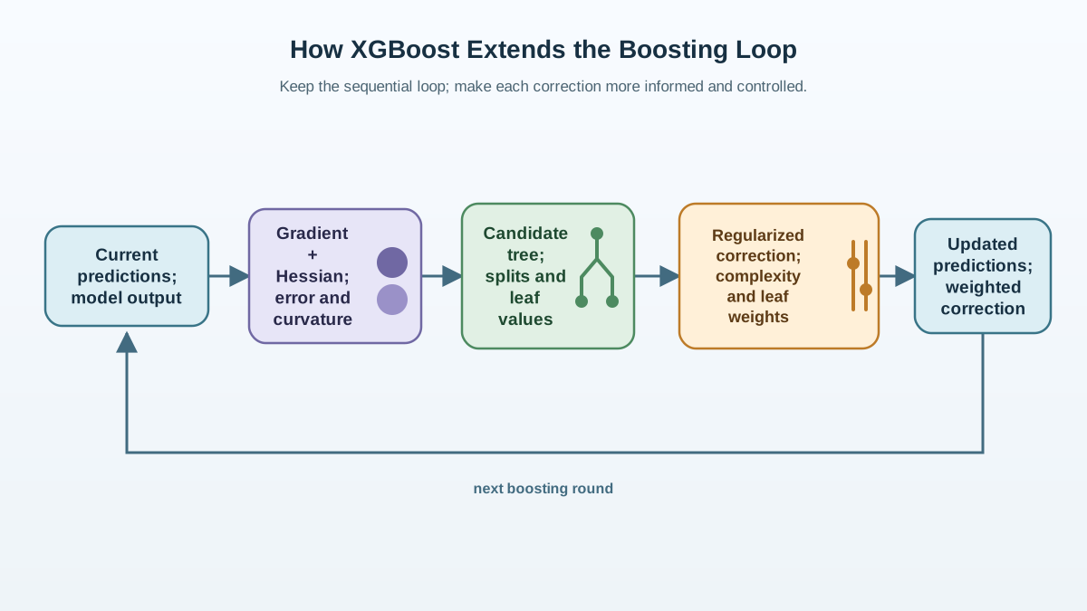
Two additions matter most, and both are worth understanding before you touch a single parameter.
Second-order optimization. Plain gradient boosting uses the first derivative of the loss function—the slope—to decide how to update its predictions. It knows which direction is downhill, but not how sharply the terrain curves. XGBoost also computes the second derivative, the Hessian, which tells it about curvature.
Here is the practical difference. Imagine walking down a hill in the dark. With only the slope, you know which way is down, but you cannot tell whether the ground is about to drop steeply or flatten out. With curvature information, you can sense when to take a smaller, safer step because the terrain is changing fast.
That curvature information flows through the whole training process. For each training example, XGBoost computes a gradient and a Hessian from the current prediction error. When it builds a candidate tree, it aggregates those values within each leaf. The aggregates help determine two things: the leaf's output value, and how much a proposed split improves the model. This is not a vague improvement—it changes concrete decisions about where to split and what value each leaf should predict.
Built-in regularization. This is the part I think beginners undervalue. A naive boosting loop will happily keep adding trees until it has memorized the training data. XGBoost adds penalty terms to its objective from the start—one that penalizes tree complexity by counting leaves, and another that shrinks the magnitude of leaf weights.
But be careful about what this means. Built-in regularization gives you useful controls, not immunity. The penalties do not automatically protect you from overfitting. They give you levers: you can penalize complexity directly, shrink leaf weights, limit tree depth, or control how many trees get added. Generalization still depends on how you set tree size, learning rate, and number of rounds—and on how you validate the result.
Common mistake: Treating XGBoost's regularization as a safety rail that makes overfitting impossible. It is a set of controls. You still have to set them thoughtfully and check performance on data the model has not seen.
Knowledge check
Check your understanding
Answer this question before you continue.
Why It Got Fast: Engineering, Not Magic
The accuracy story is only half of XGBoost's reputation. The other half is speed, and that speed comes from engineering choices worth understanding at a conceptual level.
Boosting builds trees sequentially—each tree depends on the one before it. But inside a single tree, there is plenty of parallel work available. When a tree node needs to find the best split, XGBoost can evaluate candidate split points across many features simultaneously. The trees are still built one after another; the work inside each tree is what gets parallelized.
XGBoost also uses approximate split finding. Instead of scanning every possible threshold for every feature, it can place candidate splits at quantiles of the feature distribution. This trades a small amount of precision for large speed gains on big datasets. And its cache-aware computation reduces memory pressure, which matters more than most beginners expect when datasets grow.
None of this changes the underlying learning idea. The model you get is still a boosted tree ensemble. But these optimizations are why XGBoost can handle datasets that would make a naive boosting implementation crawl.
Knowledge check
Check your understanding
Answer this question before you continue.
XGBoost vs. Plain Gradient Boosting: What Actually Changes
If you learned gradient boosting through scikit-learn's GradientBoosting classes, you have seen the plain version. Here is how it compares to XGBoost on the axes that matter:
| Plain Gradient Boosting | XGBoost | |
|---|---|---|
| Optimization | First derivative (gradient) | First and second derivative (gradient + Hessian) |
| Regularization | Minimal, external | Built into the objective |
| Training speed | Slower on large data | Parallelized, approximate splits, cache-aware |
| Typical use | Learning, small datasets | Tabular problems where measured performance justifies the complexity |
One honest complication: the line between "plain" and "XGBoost" is not perfectly sharp. Scikit-learn's newer HistGradientBoosting classes also use second-order information and parallelization, borrowing ideas from the same lineage. So the real spectrum runs from basic boosting to increasingly engineered implementations, with XGBoost near the engineered end.
Here is the takeaway I want you to keep: for many small and medium tabular datasets, the accuracy difference between a well-tuned plain boosting model and XGBoost is modest. The bigger wins are speed, sensible regularization defaults, and ecosystem maturity. Do not assume XGBoost is always more accurate just because it is more famous.
Knowledge check
Check your understanding
Answer this question before you continue.
When XGBoost Is the Right Tool—and When It Is Not
The honest answer is not a dataset-size threshold. It is a measured comparison.
Start with a baseline. A linear model or a single decision tree will tell you something valuable: how hard is this problem, really? If a simple model gets you most of the way, the extra capacity of a boosted ensemble may not be worth the complexity. If the baseline underfits badly, that is your signal to try a more expressive model.
Then test a tree ensemble on a validation design appropriate to your data. XGBoost earns its place when its improvement over simpler models justifies the extra tuning and operational complexity. That judgment depends on your problem's constraints: how much accuracy you need, how much latency you can tolerate, how much preprocessing you want to maintain, and whether anyone needs to interpret the model.
When a different boosting library fits better, use it. LightGBM is often faster on very large datasets, and CatBoost handles categorical features with less preprocessing. XGBoost is not the only option, and loyalty to a library is not a modeling strategy.
One tradeoff deserves honesty: boosted ensembles are harder to interpret than a single tree. If your problem demands explainability—regulatory reporting, medical decisions, debugging a model with a stakeholder—a single tree or a linear model may serve you better than a few extra points of accuracy.
Note: XGBoost does not remove data preparation work. Depending on the interface and version you use, its conventions for categorical features and missing values differ from scikit-learn's. Encoding choices, leakage prevention, and pipeline validation still matter—and they must be tested as part of your full cross-validation workflow, not assumed away.
Common Mistakes Beginners Make with XGBoost
I have watched beginners make the same mistakes with XGBoost repeatedly. Each one teaches something about the mechanism.
Mistake 1: Making XGBoost the default first model. If you never measure a simple baseline, you cannot tell whether boosting is actually helping. The baseline is not a formality; it is your reference point for whether the complexity is paying for itself.
Mistake 2: Cranking up the number of trees without touching the learning rate. More trees are not automatically better. With a high learning rate, many trees mean the model keeps making large corrections and eventually memorizes noise. The learning rate and the number of trees work as a pair—lower the learning rate, and you can usually afford more trees.
Mistake 3: Ignoring the regularization knobs. This one frustrates me most, because regularization is one of XGBoost's real advantages. But the point of those knobs is not that defaults protect you. It is that you have explicit control over complexity. Learn what the controls do, then set them deliberately.
Mistake 4: Assuming XGBoost handles data like scikit-learn models. Its conventions for categorical features and missing values differ from what you may be used to. Check the documentation for your specific interface and version before you assume your preprocessing pipeline transfers unchanged.
Each mistake is evidence about what the model is actually doing. Too many trees means you are memorizing instead of learning. Ignored regularization means you gave up control over complexity. No baseline means you are flying without instruments.
The Practical Decision Rule
XGBoost is not magic. It is gradient boosting with serious engineering behind it—second-order optimization for better-informed updates, built-in regularization for controlling complexity, and aggressive speed optimizations that make it practical on larger problems.
Use it when a tabular problem needs more capacity than your baseline provides, and when the measured improvement justifies the tuning and operational cost. Skip it when a simple model suffices, when interpretability matters more than accuracy, or when you are still learning what a reasonable baseline looks like.
Your next step is concrete: run a baseline on your data. Then try XGBoost. Compare them honestly on a held-out set. If boosting wins by a margin that matters for your problem, you have found your workhorse. If not, you have learned something more valuable—that your problem did not need the extra machinery.
And when you do tune XGBoost, you already know the levers that matter. The learning rate and tree depth you learned from gradient boosting still apply. You just have regularization controls in hand now, and you know what they are for.
Knowledge check
Final check
Finish the article by checking the ideas you just learned.
References
Research updated Sep 8, 2026


