
Random Forest vs Decision Tree: Why Many Weakly Related Trees Help
A single decision tree can feel like a confident liar: it nails your training data, then wobbles on new data, and reshapes its entire structure when one…

Key topics
A single decision tree can feel like a confident liar: it nails your training data, then wobbles on new data, and reshapes its entire structure when one row changes. The fix is not one better tree. It is many weakly related trees whose errors cancel out.
Why a Single Tree Wobbles
If you have worked with decision trees, you have probably seen the pattern. Train a deep tree on your data and it memorizes the training set with near-perfect accuracy. Then validation scores drop, and you realize the tree did not learn the signal—it learned the noise.
That is not a tuning failure. It is structural.
A decision tree greedily picks the best split at each node, one at a time, always chasing the largest immediate impurity reduction. That greedy search makes the tree exquisitely sensitive to whatever happens to be in the training data. A few noisy rows can tip a split decision. Once the top split changes, every split below it changes too, and you end up with an entirely different tree.
This is what statisticians call variance: the model's predictions change a lot across slightly different training sets. A deep tree has high variance because it has enough freedom to lock onto patterns that are really just noise. A shallow tree has lower variance but higher bias—it cannot capture the real structure either.
So you face an uncomfortable trade. Deep trees overfit. Shallow trees underfit. And anywhere in between, the tree structure itself remains fragile: change a handful of rows and the whole diagram redraws.
Knowledge check
Check your understanding
Answer this question before you continue.
The Ensemble Idea: Average Out the Noise
Here is the intuition that changes everything: if one tree's mistakes are partly random, then many trees' mistakes should partially cancel out.
But there is a catch. If you train many trees on the same data, they all see the same noise. They make the same mistakes. Averaging them changes nothing. You need trees that disagree—trees that each saw a slightly different version of the world.
That is exactly what bagging (short for bootstrap aggregating) provides. Instead of training every tree on the full dataset, you draw a random sample with replacement for each tree. Some rows appear multiple times in a tree's training set; others never appear at all.
Each tree in the bagged ensemble is trained on its own slightly distorted view of the data. One tree might never see the three most unusual customers. Another tree might see them three times each. As a result, the trees make different mistakes, and when you average their predictions, those individual errors start to cancel.
This is the core mechanism of bagging machine learning: averaging many high-variance models lowers the overall variance without raising bias much. The forest generalizes better not because each tree is smarter, but because the crowd is more stable than any single member.
Knowledge check
Check your understanding
Answer this question before you continue.
Feature Randomness: Why Trees Must Disagree
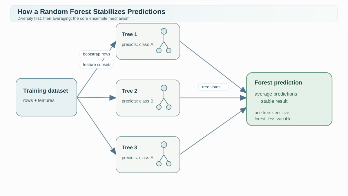
Bagging alone is not enough. Here is why.
Most datasets have a few strong features that dominate the split decisions. If you bag a hundred trees but every tree keeps splitting on the same two or three powerful features, your trees are still highly correlated. They disagree less than you hoped, and their errors do not cancel as cleanly.
The random forest algorithm solves this with a second injection of randomness: feature randomness (also called feature bagging). At each split, the tree does not consider all features. It randomly selects a subset and only searches for the best split among those candidates.
In scikit-learn, the max_features parameter controls how many features each split may consider. For classification, a common default is the square root of the total feature count. For regression, it is often a third of the features. The exact value matters less than the mechanism: no single feature can dominate every tree, because most trees never even get to look at it for a given split.
This is what makes a random forest a true ensemble rather than a bag of near-identical trees. Bootstrap sampling decorrelates the trees by changing which rows they see. Feature randomness decorrelates them by changing which features they can use. Together, they produce many weakly related trees whose errors are less correlated—and therefore average out more cleanly.
That is the random forest explained in one sentence: many trees, each trained on a different sample of rows and a different sample of features, whose averaged predictions are more stable than any individual tree's guess.
Knowledge check
Check your understanding
Answer this question before you continue.
Decision Tree vs Random Forest: The Tradeoff Table
The practical question is not which model is "better." It is which tradeoff you can afford.
| Decision Tree | Random Forest | |
|---|---|---|
| Variance / overfitting | High, especially with deep trees | Lower, because averaging cancels individual tree errors |
| Interpretability | High—you can draw and trace the full path | Low—no single diagram explains the ensemble |
| Training cost | Fast, even on large data | Slower, since you train many trees |
| Prediction cost | Lower | Higher, since every tree must predict |
| Stability to data changes | Fragile—one row can redraw the tree | Stable—individual trees change but the average barely moves |
| Many features | Greedy splits favor strong features | Feature randomness spreads influence across features |
| Feature importance | Noisy and unstable | More stable, averaged across many trees |
The single tree wins where explanation matters more than peak accuracy. It is fast, visual, and readable: you can show a stakeholder exactly which rules produced a prediction. The forest wins where generalization matters more than a readable path. It is slower and opaque, but it holds up better on unseen data.
A forest is not always the right answer. On a small, clean dataset with a handful of meaningful features, a single tree can perform perfectly well and save you the complexity. Do not reach for a hundred trees when ten rules tell the whole story.
Feature Importance: What the Forest Can and Cannot Tell You
One practical payoff of the forest deserves special attention: feature importance.
A single tree's feature importance is noisy. Because the tree structure itself is unstable, the importance scores it produces are unstable too. One tree might rank a feature first because it happened to grab that feature at a lucky split; another tree trained on slightly different data might barely use it.
A random forest averages importance across many trees, and that averaging produces a more stable ranking of which features matter. In scikit-learn, the feature_importances_ attribute measures how much each feature reduces impurity across all the splits in the forest. The more a feature helps separate the data, the higher its score.
That stability is real, but do not confuse it with validity. Impurity-based importance reflects how often and how effectively a feature was used inside this particular model—not an objective measure of how much a feature matters in the world. With correlated features, the forest may split unevenly between two equally useful predictors, making one look far more important than the other. The ranking is also influenced by how many split opportunities each feature received, which depends on max_features and the data.
So treat feature_importances_ as a screening signal, not a verdict. If interpretation genuinely matters, compare it with permutation importance computed on held-out data, which measures how much predictions degrade when you shuffle one feature at a time. And remember the deeper warning: feature importance reflects predictive usefulness inside your model, not causal effect. A feature can rank high because it correlates with the real driver, not because it causes the outcome.
How to Choose: A Practical Decision Rule
Here is the decision rule I use.
Use a single tree when you must show and explain the exact decision path, your dataset is small and clean, or you need a fast baseline before investing in anything fancier. If a stakeholder needs to see the rules, a single tree is the only model that can honestly show them.
Use a random forest when you care most about generalization and you can afford the compute. Noisy or high-dimensional data are situations where the forest is worth testing—not an automatic recommendation. The real test is measured: does the forest beat the tree on held-out or cross-validated data by enough to justify losing the readable path?
There is also a useful middle path. Train a forest to get stable feature importance and good generalization. Then, when you need a readable story, train a single shallow tree and inspect its structure. The shallow tree will not match the forest's accuracy, but it can give you a human-readable approximation of the patterns the forest found.
A forest still needs tuning—number of trees, max_features, depth limits—but its defaults are reasonable starting points. Start with a few hundred trees, check whether validation performance plateaus, and adjust from there. Whatever you choose, validate: the forest reduces variance, but it can still overfit, especially with deep trees on small or noisy data.
Knowledge check
Check your understanding
Answer this question before you continue.
Your Next Step
Do not take this on faith. Run the comparison yourself.
Train a single deep decision tree and a random forest on the same dataset. Compare their training scores against their validation scores. Here is the hypothesis worth testing: the tree will show a large gap—high training accuracy, lower validation accuracy—while the forest will show a smaller gap, because averaging has smoothed away much of the noise the tree memorized.
But measure it. The forest can still overfit, and the gap alone does not tell you which model actually generalizes better. Trust held-out or cross-validated performance as the primary signal, and use the training-validation gap as supporting evidence.
Then inspect the forest's feature importance and ask whether the ranking matches what you know about the data. If it does, you have just seen the ensemble mechanism working with your own data.
The durable takeaway is this: a random forest trades a readable single path for a more stable, generalizing answer. The choice between a decision tree and a random forest is not about which algorithm is smarter. It is about what you need to explain versus how well the model must hold up on data it has never seen.
Knowledge check
Final check
Finish the article by checking the ideas you just learned.
References
Research updated Sep 8, 2026


