
Gaussian Mixture Models for Clustering: Soft Groups With Probabilities
Picture a point sitting exactly between two well-separated blobs of data. K-means will force it into one group or the other, even when the data could…

Key topics
Picture a point sitting exactly between two well-separated blobs of data. K-means will force it into one group or the other, even when the data could plausibly have produced it from either side. That forced choice is not a minor annoyance—it is a symptom of a deeper assumption. K-means treats a cluster as a hard-edged region around a center. Gaussian mixture models replace that picture with something more honest: clusters as overlapping probability distributions, with every point carrying a membership score instead of a single label.
The Problem K-Means Leaves Unanswered
If you have worked with K-means, you already know its rhythm: pick k centers, assign each point to the nearest one, recompute the centers, repeat. The output is clean. Every point gets exactly one label.
That cleanliness is also the limitation. K-means has no way to say "this point is ambiguous." It only measures distance to a centroid, so a point straddling the boundary between two dense regions gets assigned to whichever center happens to be a hair closer. The underlying mental model is that a cluster is a hard-edged sphere around a center, and membership is binary: in or out.
Real data rarely cooperates with that picture. Clusters overlap. They stretch. They have different sizes and densities. And some points genuinely sit in the gray zone between groups.
Gaussian mixture models clustering starts from a different question. Instead of asking "which group is this point nearest to?", it asks "which mixture of probability distributions most plausibly generated this point?" That reframe changes what you get back: not just labels, but probabilities, elliptical cluster shapes, and a generative story about how the data came to exist.
Clustering as a Mixture of Gaussians
Start with the building block. A single Gaussian distribution models one blob of data with two ingredients: a mean, which locates the center, and a covariance, which describes how the blob spreads out in each direction. In two dimensions, a Gaussian looks like an ellipse. In higher dimensions, it is an ellipsoid.
A Gaussian mixture model stacks several of these blobs together. Each component has its own mean, its own covariance, and a mixing weight. The mixing weight represents the relative size of the component under the fitted model—how much of the data it accounts for compared to the others. A component with weight 0.6 accounts for roughly 60 percent of the data according to the model; a component with weight 0.1 is a smaller population.
The generative story makes this concrete. Imagine creating a synthetic dataset from the model. First, pick a component by rolling a die weighted by the mixing weights. Then draw a point from that component's Gaussian distribution. Repeat thousands of times, and you get a dataset that looks like a collection of overlapping elliptical blobs.
That generative framing is the key insight—but it comes with an important caveat. The model imagines a hidden component that generated each point. That component identity is a latent variable: an assumption the model makes to explain the data, not a recovered fact about the world. A GMM is fundamentally a density model—a description of the probability distribution that produced your data. Clustering is one use of that model, not the whole point of it. When you fit a GMM, you are estimating the parameters of several Gaussians whose weighted sum approximates your data's distribution. The clusters fall out of that estimate.
Knowledge check
Check your understanding
Answer this question before you continue.
Soft Assignments: Membership as Probability, Not a Label
Once the model is fitted, every point gets a set of responsibility scores. For each component, the model computes the probability that this point belongs to it, given the fitted components and their weights. A point near the heart of one component might carry a 0.98 score for that component and near-zero for the others. A point in the overlap zone between two components might split its score 0.55 and 0.45.
This is soft clustering. You can recover hard labels by taking the component with the highest score—the argmax—but you lose information when you do. The scores tell you something the hard label hides: how much this point sits in the gray zone between the fitted components.
That information is practically useful. If you sort points by their maximum membership score, the low scorers are your ambiguous cases. They deserve inspection, not blind trust. A point with a top score of 0.51 is the model saying "this is my best guess, but the other component explains this point almost as well." Treating it with the same certainty as a point at 0.99 is throwing away the very advantage GMM gives you.
Common mistake: Reading a high membership score as proof that a point truly belongs to a real-world group. The score only says the point fits this Gaussian well relative to the other fitted components. If the model's assumptions are wrong—wrong component count, wrong covariance structure, poorly scaled features—the score can be confidently misleading. These are model-relative responsibilities, not calibrated real-world probabilities.
Knowledge check
Check your understanding
Answer this question before you continue.
Covariance: Where GMM Earns Its Keep
K-means tracks only centers. That single choice imposes a hidden geometric assumption: clusters are roughly spherical and similarly sized. When your data contains elongated or elliptical clusters, K-means will slice through them at awkward angles, because it has no vocabulary for shape.
GMM tracks a covariance matrix for each component, and that changes everything. A component can stretch along one axis and stay narrow along another. It can tilt at an angle. It can be large and diffuse or small and tight. The covariance matrix is what lets GMM model elliptical and overlapping clusters that a single K-means partition cannot represent.
Scikit-learn's GaussianMixture class exposes this flexibility through the covariance_type parameter, and the choice is a real tradeoff:
full: each component gets its own unrestricted covariance matrix. Maximum flexibility, but the most parameters to estimate.tied: all components share the same covariance matrix. A middle ground that assumes similar shapes across clusters.diag: each component has its own covariance, but only along the axes—no rotation. Cheaper to estimate, but clusters must align with the feature axes.spherical: each component is a sphere with its own radius. The closest to K-means' implicit assumption, but still probabilistic.
Full covariance is the most flexible, but flexibility has a price. Each component needs enough points to estimate its covariance reliably. When a component has too few points, the estimation can collapse, and the likelihood can diverge toward infinity as the Gaussian shrinks to a razor-thin sliver around a single point. Scikit-learn applies regularization to mitigate this, but the real fix is more data per component or a simpler covariance structure.
Knowledge check
Check your understanding
Answer this question before you continue.
How the Model Is Fit: Expectation-Maximization in Plain Terms
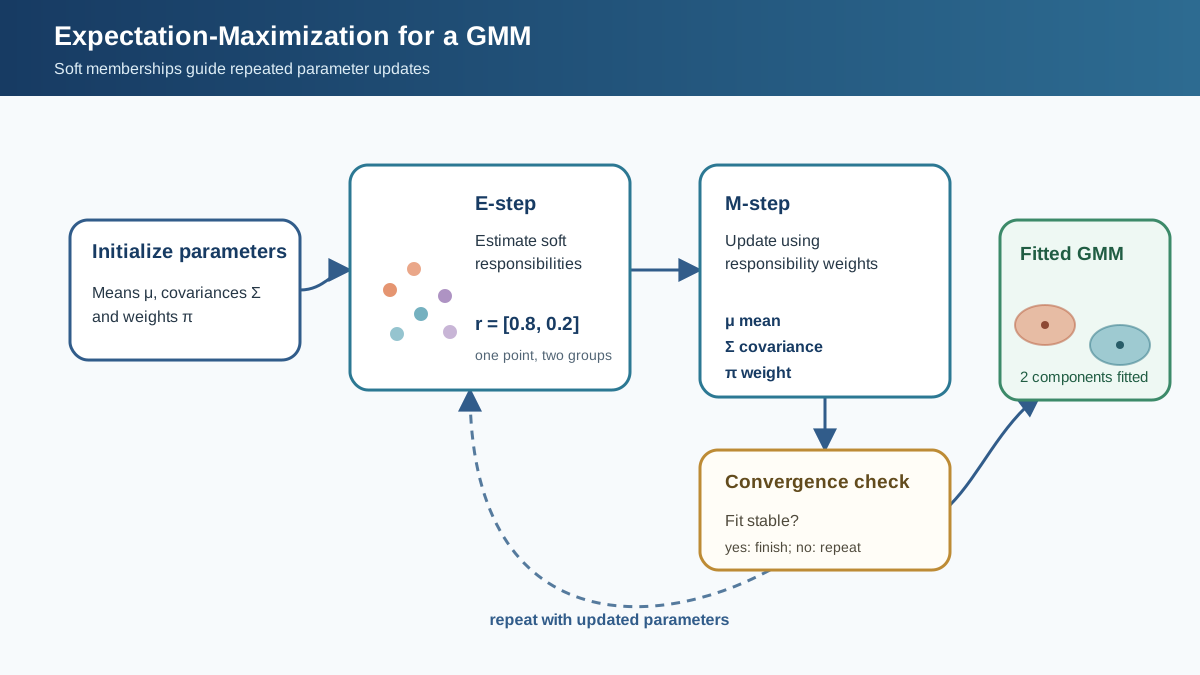
GMM parameters are estimated by an algorithm called expectation-maximization, or EM. If you have seen K-means converge, the shape of EM will feel familiar—it is the same guess-and-refine loop, with one crucial difference.
The loop alternates two steps. In the E-step, the algorithm takes the current component parameters and computes each point's membership scores across all components. In the M-step, it re-estimates each component's mean, covariance, and mixing weight, using every point but weighting each point's contribution by its membership score from the E-step. Repeat until the log-likelihood stops improving meaningfully.
The difference from K-means is the weighting. K-means commits each point to exactly one cluster during its assignment step. EM lets every point contribute to every component, but in proportion to its score. A point that is 90 percent component A and 10 percent component B nudges A's parameters strongly and B's parameters barely at all.
Initialization matters here just as it does with K-means. EM can converge to a poor local optimum, and different starting points can lead to different solutions. The standard safeguard is to run multiple initializations and keep the best fit. In scikit-learn, the n_init parameter controls this, and the default initialization uses the K-means++ strategy to pick sensible starting centers.
When GMM Fits—and When It Does Not
Choosing a clustering method is choosing a set of assumptions. Here is how I think about the decision.
Choose GMM when each group can plausibly be represented by an elliptical density with its own spread, when clusters overlap, and when membership scores would help you interpret the result. The covariance structure gives you shape flexibility that centroid-based methods lack, and the soft assignments give you ambiguity information that hard clustering discards.
Choose K-means when your clusters are roughly spherical and well separated, and when speed and simplicity matter more than probabilistic nuance. K-means scales to very large datasets more easily and has fewer parameters to worry about.
Choose DBSCAN when density connectivity is the primary concept—when you expect arbitrary shapes, strongly varying density, or a meaningful set of noise points. GMM forces every point into the mixture; there is no "noise" component unless you build one in. DBSCAN explicitly labels low-density points as noise, which is the right tool when your data contains outliers you do not want dragging your cluster parameters around.
The boundary between GMM and DBSCAN comes down to what "different sizes" means. GMM handles components with different Gaussian spreads—one group tightly packed, another more diffuse. But when groups are connected by dense bridges or shaped like crescents and rings, a density-based view serves you better than any number of elliptical components.
| Method | Core assumption | Output | Shape flexibility | Noise handling | Parameter cost |
|---|---|---|---|---|---|
| K-means | Spherical, similar-sized clusters | Hard labels | Low | Poor—outliers drag centroids | Lowest |
| GMM | Gaussian-shaped components | Probabilities + hard labels | High—elliptical, tilted, varied size | Poor—outliers affect parameters | Higher—covariance matrices add parameters |
| DBSCAN | Dense regions separated by sparser space | Labels + noise flag | Very high—arbitrary shapes | Explicit noise labeling | Moderate |
GMM's core assumption is also its boundary. If your clusters are crescent-shaped, ring-shaped, or heavily skewed, no number of Gaussian components will model them well. You can approximate a crescent with many small components, but that is a patch, not a solution. And unlike DBSCAN, GMM is not robust to outliers—a stray point far from the main mass can pull a component's mean and inflate its covariance.
Knowledge check
Check your understanding
Answer this question before you continue.
Reading the Probabilities With a Skeptical Eye
The probabilistic output of GMM looks rigorous. It is easy to mistake that rigor for proof that the groups are real.
It is not. A membership score of 0.97 means "this point fits this Gaussian well relative to the other fitted components." It does not mean "this group corresponds to a genuine category in the world." The model can be confidently wrong when the Gaussian assumption is violated, when the number of components is wrong, or when the data contains structure the model cannot represent.
Choosing the number of components is a model-selection problem, not a visual guess. You cannot reliably eyeball a two-dimensional plot and pick the right k when your data lives in higher dimensions. Information criteria and cross-validation help, but they are tools for comparing models, not proof that any of the models is true.
Warning: Soft probabilities are not a license to skip validation. They are an invitation to inspect more carefully. Use the scores to surface ambiguous points and drive investigation, then apply the same domain checks and stability tests you would use on any clustering result. A neat probabilistic output can be just as misleading as a neat plot.
When you fit a GMM, work through the output in three passes. First, inspect the fitted components themselves: their means, covariance shapes, and mixing weights. Do the component geometries match what you know about the domain, or is the model contorting itself to fit noise? Second, look at the responsibility patterns—which points have low maximum scores, and do they cluster in specific regions of the feature space? Those regions are where the model is least decisive, and they deserve the most scrutiny. Third, test sensitivity: rerun the fit with different initializations, different component counts, and different covariance types. If the groups reshuffle dramatically under small changes, the structure is not stable enough to interpret.
The honest way to use GMM is as a tool for surfacing structure worth questioning. Fit the model. Look at which points carry low scores. Ask whether the components correspond to something meaningful in your domain. Run the model on perturbed data and see whether the groups survive. The probabilities make the model's ambiguity visible—that is their value. The validation mindset is what keeps that ambiguity from becoming overconfidence.
Start with a two-component fit on a small dataset you understand well. Compare the full and diagonal covariance structures. Look at which points flip between components and which stay firmly anchored. That contrast will teach you more about what GMM's probabilities actually mean than any abstract explanation—and it will show you exactly where the model's confidence deserves your skepticism.
Knowledge check
Final check
Finish the article by checking the ideas you just learned.
References
Research updated Sep 8, 2026


