
Classical Anomaly Detection: Find Unusual Data Without Labels
Anomaly detection is not "find the weird rows." It is a decision about what counts as normal, made before you ever run an algorithm. Get that decision…

Key topics
Anomaly detection is not "find the weird rows." It is a decision about what counts as normal, made before you ever run an algorithm. Get that decision wrong, and your alerts will flag the wrong records with perfect confidence.
Here is the trap: every classical method quietly assumes a definition of "normal." Robust covariance assumes normal data lives in an elliptical cloud. Isolation Forest assumes anomalies are easy to separate with a few random cuts. Local Outlier Factor assumes normal points have neighbors that look like them. When your data violates the assumption, the method does not fail loudly. It fails quietly, producing alerts that look reasonable and mean nothing.
The fix is not to find a better algorithm. It is to frame the problem correctly first.
Why "Find the Weird Rows" Is the Wrong Starting Point
Most people come to anomaly detection with a simple mental model: run an algorithm, get a list of unusual records, investigate them. That model skips the only question that actually matters: what does "normal" mean in your data?
Consider a manufacturing sensor dataset. Is a reading normal because it falls within a familiar range? Because it resembles readings from the same machine at the same time of day? Because it sits in a dense neighborhood of similar readings? Each of those definitions points to a different method, and each method can flag a different set of records on the same data.
The practical question is never "is this point unusual?" It is "is this point unusual in a way that matters for my problem?" A rare but legitimate transaction is unusual. It is not bad. A sensor spike during a scheduled maintenance window is unusual. It is not a failure. Rare does not equal erroneous, and confusing those two ideas is the most expensive mistake in this field.
That is why anomaly detection is best treated as an unsupervised investigation: you are generating hypotheses about which records deserve human attention, not producing a verdict about which records are wrong.
Knowledge check
Check your understanding
Answer this question before you continue.
Outlier Detection vs. Novelty Detection: Two Different Questions
Before choosing a method, answer one question: is your training data already polluted, or is it clean?
Scikit-learn draws the line sharply, and the distinction changes which estimators you can use.
Outlier detection assumes your training data already contains anomalies. The estimator tries to fit the dense, concentrated regions of the data while ignoring the deviant points. You use this when you have a messy dataset and want to clean it, or when you suspect contamination but cannot identify it by hand.
Novelty detection assumes your training data is clean and trustworthy. The question changes from "which points in this mess are strange?" to "does this new observation come from the same distribution as my trusted baseline?" You fit on the clean data, then score new records as they arrive.
The practical consequence is direct. Outlier detection is for cleaning a messy dataset you already have. Novelty detection is for flagging new records against a baseline you trust. If you fit a novelty detector on polluted data, the "normal" boundary shifts to include the contamination. If you fit an outlier detector on clean data, you will flag healthy records that merely sit at the edges of a legitimate distribution.
This geometry problem—defining what is close and what is far—is the same one you wrestle with in clustering. The difference is that clustering asks "what groups exist here?" while anomaly detection asks "what does not belong to any group?"
Knowledge check
Check your understanding
Answer this question before you continue.
Four Classical Methods and the Assumption Each One Makes
Once you know whether you are doing outlier or novelty detection, the next question is which geometric assumption fits your data. Scikit-learn gives you four main tools, and each one encodes a different bet about the shape of normal.
| Method | Assumption About Normal Data | When It Works | When It Fails |
|---|---|---|---|
| Robust Covariance (Elliptic Envelope) | Normal data lives in an elliptical region | Clean, roughly Gaussian, unimodal data | Multimodal or heavily skewed normal data |
| One-Class SVM | A boundary can separate normal from everything else | Clean training data with a tight boundary needed | High dimensions; very large datasets |
| Local Outlier Factor (LOF) | Normal points have neighbors with similar local density | Varied-density data where local context matters | When global density differences are the signal |
| Isolation Forest | Anomalies are easy to isolate with few random splits | Large, messy datasets; few shape assumptions | When anomalies hide inside dense normal regions |
Robust Covariance fits an ellipse to the concentrated center of your data, ignoring points that stretch the shape. It is fast and interpretable, but it assumes your normal data is roughly Gaussian and unimodal. If your normal data has two distinct modes—say, transactions from two very different customer segments—the ellipse will cover empty space between them and flag legitimate points at the edges of each mode.
One-Class SVM learns a boundary around your concentrated data rather than assuming a shape. It is flexible, but that flexibility comes with sensitive kernel and gamma parameters. In higher dimensions, it struggles: the boundary has too much freedom and can hug individual points instead of the actual distribution.
Local Outlier Factor scores each point by comparing its local density to its neighbors'. A point is anomalous if its neighborhood is sparse relative to the neighborhoods around it. This makes LOF strong when your data has regions of naturally different density—a point that is unusual for its neighborhood gets caught even if it sits in a globally dense area.
Isolation Forest takes a different path entirely. Instead of modeling normal data, it tries to isolate each point with random splits. Anomalies are easy to separate, so they need few splits. Normal points require many cuts to isolate. It is fast, scales well, and makes few assumptions about shape, which makes it a sensible baseline for larger, messier datasets.
No method wins everywhere. Simulation studies consistently show that performance varies with dataset characteristics, which means the choice should be deliberate, not habitual.
Knowledge check
Check your understanding
Answer this question before you continue.
Scaling, Geometry, and the Curse of Dimensionality
Here is where anomaly detection silently breaks. Distance-based and density-based methods—LOF, One-Class SVM, Robust Covariance—are brutally sensitive to feature scale. If one feature ranges from 0 to 1 and another ranges from 0 to 10,000, the second feature dominates every distance calculation. The first feature might as well not exist. Standardize your features before fitting these methods.
Isolation Forest is different. Because it works on splits rather than distances, scale does not distort its geometry the same way. Standardizing is not a free requirement here—and if your features carry meaningful units or thresholds, forcing them onto a common scale can actually blur the structure the forest would otherwise exploit. My rule: scale for distance-based, kernel, covariance, and density methods. For Isolation Forest, decide deliberately rather than by habit, and test both representations when scale sensitivity matters.
High dimensions are a deeper problem. As dimensionality increases, distances between points converge. Everything becomes roughly equidistant from everything else, and every point starts to look equally isolated. This is not a parameter you can tune away. It is a property of high-dimensional space.
Dimensionality reduction can help, but it carries a specific danger: compressing variance can discard the very variation that defines an anomaly. If a rare failure mode lives in a low-variance direction, PCA will happily drop it. Reduce dimensions with the anomaly question in mind, not just for visualization convenience.
Knowledge check
Check your understanding
Answer this question before you continue.
Choosing a Method: A Decision Rule, Not a Menu
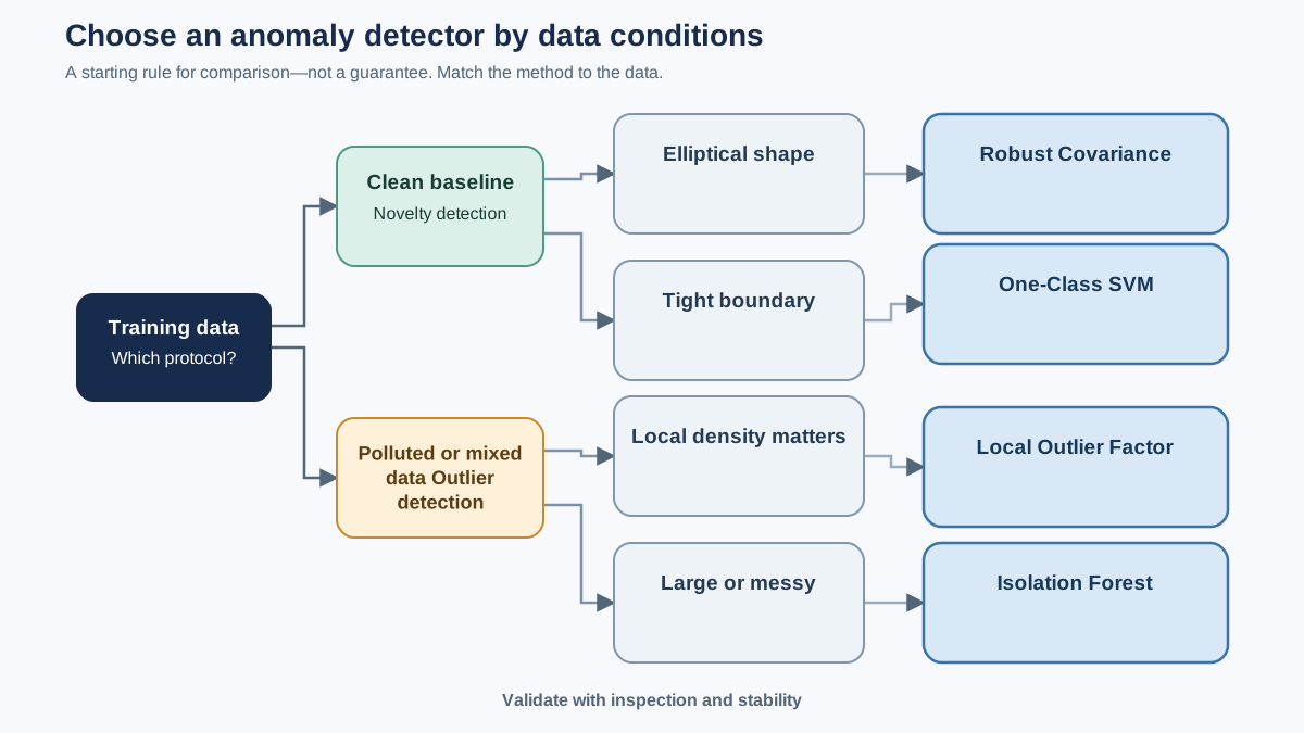
You do not need a flowchart. You need four criteria and a default.
Ask yourself: What shape does normal data take? How large is the dataset? How many dimensions? Is the training set clean or polluted? And most importantly, what does a false alert cost compared to a missed anomaly?
Here is how I would decide:
- Robust Covariance for clean, roughly Gaussian data when you want a fast, interpretable baseline.
- Isolation Forest as a practical baseline for larger, messier datasets where you do not trust shape assumptions.
- Local Outlier Factor when local density variation matters—when a point can be unusual relative to its neighborhood even in a globally dense region.
- One-Class SVM when you have clean training data and need a tight, flexible boundary, and your dataset is small enough to make the fit practical.
And here is when not to use each: do not use Robust Covariance on multimodal or heavily skewed normal data. Do not expect One-Class SVM to scale gracefully to very large datasets. Do not trust LOF when your data has one global density and you care about global outliers.
Run two or three detectors and compare their alert sets. Records flagged by multiple methods deserve earlier inspection—but agreement is prioritization evidence, not validation. Methods can share the same feature flaws, scaling choices, or blind spots. A record flagged by only one detector may still matter if that detector sees a structure the others cannot.
Contamination: The Number You Must Not Guess
The contamination parameter is one of the most consequential settings in classical anomaly detection, and the most mishandled. But before you tune it, you need to understand what it actually does.
In scikit-learn, contamination is an assumed fraction of anomalies used by some estimators to set a threshold on their training data. It directly controls how aggressive the alerting is. The default is often a small fixed value, which silently assumes your data is mostly clean.
Novelty detection changes the protocol. Instead of assuming a polluted training set, you fit on a clean baseline and score new observations against it. The question is not "what fraction of this mess is bad?" but "does this new record come from the same distribution I trusted?" Check each estimator's documented scoring and threshold behavior rather than assuming contamination behaves identically everywhere.
Set contamination too high and you flag normal records. Set it too low and you miss real anomalies. The uncomfortable truth is that you rarely know the true contamination rate. Treat it as a tuning lever tied to the cost of false alerts, not as a fact about the data.
The practical pattern: fit with a range of contamination values and inspect how the alert set changes. If the same records keep getting flagged across a range of settings, those are your strongest candidates. If the alert set reshuffles completely with every small change, the signal is weak and the parameter is doing the work, not the data.
From Scores to Alerts: The Review Queue
Most anomaly detectors do not hand you truth. They hand you a score or a ranking. The binary label appears only after you choose a cutoff—and that cutoff is a business decision, not a statistical one.
Think of it as a review queue. You have limited investigation capacity: a fraud team can examine so many transactions per day, an engineer can inspect so many flagged sensor readings per hour. Your contamination setting or score threshold should reflect that capacity and the relative cost of a false alert versus a missed anomaly.
When you inspect a flagged record, record what you find. A simple table works: record ID, detector scores or ranks, the feature values that made it unusual, surrounding context, and the investigation outcome. Over time, that table becomes your ground truth substitute. It tells you which detectors earn their alerts and which ones cry wolf.
Validating Alerts Without Ground Truth
Without labels, you cannot compute precision or recall. You have three tools instead: inspection, stability, and agreement.
Inspect the flagged records directly. Do they share a plausible story? Do they cluster around a particular time, a particular machine, a particular customer segment? Or are they scattered without a pattern? A coherent story is weak evidence, but it is evidence. No story at all is a warning sign.
Check stability. Does the same detector flag roughly the same records across different random seeds or subsamples? An unstable alert set means your detector is chasing noise.
Compare detectors. Agreement across methods with different geometric assumptions is the closest thing to ground truth you will get without labels—but treat it as a prioritization signal, not proof. Shared flags deserve earlier inspection. Unique flags may still be important if one detector sees a structure the others miss.
When you do have a few labels—even a handful of confirmed cases—use them. Precision and recall against those labels beat any unsupervised score.
The hard rule: an alert is a hypothesis to investigate, not a verdict. Rare data is not automatically bad data.
Common Mistakes That Produce Confident Wrong Answers
Audit your workflow against these five failure modes before you trust any output.
Mistake 1: Treating every flagged point as an error to delete. Many anomalies are legitimate rare events worth investigating. Deleting them destroys signal. Flag first, investigate second, delete only with justification.
Mistake 2: Fitting a novelty detector on polluted data, or an outlier detector on clean data. The mismatch is invisible unless you check. Know which question you are asking before you fit.
Mistake 3: Scaling without thinking. Distance-based methods need standardized features. Tree-based methods do not, and forcing a common scale can blur meaningful thresholds. Match your preprocessing to the mechanism.
Mistake 4: Trusting a single detector's score as ground truth. Compare methods, inspect alerts, check stability. A score from one model is a suggestion, not a fact.
Mistake 5: Ignoring contamination and accepting the default. The default is a guess about your data. Make the guess deliberately, and test how much it matters.
The Workflow That Survives Contact With Real Data
Here is the compact workflow I use, and the one I would start with on any unlabeled tabular dataset:
- Decide whether you are cleaning a polluted dataset or scoring new records against a clean baseline.
- Scale features for distance-based, kernel, covariance, and density methods. Decide deliberately for Isolation Forest.
- Reduce dimensions only if the anomaly question survives the compression.
- Fit two or three detectors with a range of contamination values.
- Compare the alert sets across methods and contamination settings.
- Build a review queue: rank records by how consistently they are flagged, then inspect the top of that queue within your investigation budget.
- Record what you find. If inspection reveals a legitimate subgroup your baseline never anticipated, segment the data and refit rather than deleting the subgroup.
Anomaly detection is the sibling of clustering. Both share the same geometry problem, the same scaling discipline, the same validation struggle, and the same temptation to mistake algorithm output for ground truth. Resist that temptation, and the methods will serve you well. Give in to it, and you will get confident wrong answers every time.
Start with one messy dataset you actually care about. Fit an Isolation Forest and a Local Outlier Factor. Compare their rankings, inspect the top ten records from each, and ask whether the story they tell matches what you know about the data. That single pass will teach you more about anomaly detection than reading about ten more algorithms.
Knowledge check
Final check
Finish the article by checking the ideas you just learned.
References
Research updated Sep 8, 2026


