
DBSCAN Clustering Explained: Find Dense Groups and Mark Noise
You learned K-means, and it felt clean: pick a number of groups, let centroids pull points inward, and read off the labels. Then you hit a dataset with…

Key topics
You learned K-means, and it felt clean: pick a number of groups, let centroids pull points inward, and read off the labels. Then you hit a dataset with crescents, rings, or stray outliers, and the whole tidy picture fell apart. K-means forced every point into a round group, outliers dragged centroids around like dead weight, and you had to guess k before the algorithm did any real work.
DBSCAN removes both constraints—no cluster count required, no spherical assumption. But it trades them for two knobs, eps and min_samples, that quietly decide everything. The real lesson is that DBSCAN does not find clusters. It finds regions of similar density and calls everything else noise.
Why K-Means Leaves You Wanting a Different Tool
K-means assigns every point to the nearest centroid. That single rule creates two structural problems.
First, outliers get absorbed. A point floating far from any real group still receives a label because K-means has no concept of "none of the above." The outlier drags the centroid toward it, distorting the cluster boundary for every legitimate member.
Second, K-means assumes convex, roughly equal blobs. It minimizes within-cluster distances to a center, which works beautifully for compact spheres and poorly for anything shaped like a crescent, a ring, or a long winding corridor. The algorithm cannot represent those geometries because its objective function has no way to encode them.
DBSCAN answers a different question entirely. Instead of asking "which centroid is nearest?", it asks "is this point in a dense enough neighborhood to belong to a group?" That shift from distance-to-center to local density is what lets DBSCAN find arbitrary shapes and mark outliers as noise.
The trade should be clear: DBSCAN removes the need to pick k, but asks you to define density instead.
Knowledge check
Check your understanding
Answer this question before you continue.
The Core Idea: Density, Not Distance to a Center
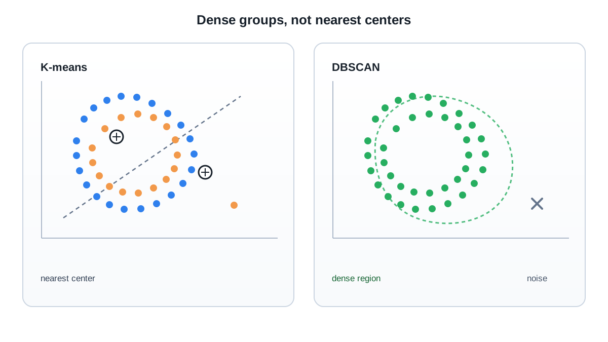
Picture a festival crowd. People cluster around food stalls and stages, packed shoulder to shoulder, while a few stragglers stand alone in the open field between them. The dense pockets are your clusters. The sparse space between them is what separates one group from another.
That image captures the mechanism of density-based clustering. A cluster is a connected region where points are packed closely enough, and sparse gaps are what divide one group from the next.
DBSCAN grows a cluster outward from any point that has enough neighbors within a fixed radius. Start at a crowded point, absorb its neighbors, then check whether those neighbors are crowded too. If they are, keep expanding. If not, stop. The cluster boundary forms where density drops below your threshold.
The analogy holds until you ask one question: what counts as "crowded"? Density is not an absolute property of the data. It is defined by the radius you choose and the minimum neighbor count you demand. Change either one, and yesterday's dense region becomes today's sparse scatter.
The Two Knobs: eps and min_samples
DBSCAN takes two parameters that define density, and both deserve your attention before you run anything. The distance metric you choose also matters, but eps and min_samples are the pair that controls what the algorithm sees.
eps is the neighborhood radius: the maximum distance within which two points count as neighbors. It is not a cap on cluster size. Clusters can chain far beyond a single radius, as long as each step finds another dense neighborhood within reach. Think of it as the arm length that determines who you can touch directly, not the total size of the crowd you can eventually reach through a chain of handshakes.
min_samples is the minimum number of points a neighborhood must hold for its center to count as a core point. The count includes the point itself. Raise it, and DBSCAN demands denser regions, labeling more points as noise. Lower it, and sparse regions can form clusters.
The failure modes are symmetric:
epstoo small fragments data into many tiny clusters and noise.epstoo large merges distinct groups into one blob.min_samplestoo high labels legitimate sparse regions as noise.min_samplestoo low lets random scatter form clusters.
The two parameters are not independent dials. They work as a pair: eps decides who is within reach, and min_samples decides whether that reach contains enough points to count as dense. A good way to think about them is that min_samples sets your strictness about noise, while eps sets the physical scale of the neighborhoods you are willing to call dense.
For a first experiment in two dimensions, min_samples around 4 or 5 is a reasonable seed. Treat it as a starting point for observation, not a rule. The real test is what happens to the noise fraction and cluster stability as you move it. In higher dimensions, density becomes harder to define reliably, so rather than blindly scaling the number up, ask whether distances between points still carry meaning at all.
Knowledge check
Check your understanding
Answer this question before you continue.
Core, Border, and Noise: The Three Labels
Every point in a DBSCAN run receives one of three labels, and understanding the difference lets you predict what the algorithm will do before you run it.
Core points have at least min_samples neighbors inside eps. They can seed a cluster and extend it outward.
Border points sit within eps of a core point but do not have enough neighbors themselves. They join the cluster but cannot extend it. They are the edge of the crowd—close enough to belong, too isolated to pull anyone else in.
Noise points are neither core nor within reach of a core point. DBSCAN labels them -1.
Watch a small example. Suppose min_samples is 4. Point A has six neighbors inside eps, so it is core. Those neighbors include point B, which has only two neighbors—not enough to be core, but close enough to A to join the cluster. B is a border point. The cluster expands through A's core neighbors, each of which may pull in their own border points, until no core point remains unvisited. Point C, sitting far from everyone, never falls inside anyone's eps neighborhood. It is noise.
One subtlety trips up many beginners: a point first marked noise can later be absorbed into a cluster. DBSCAN visits points in some order, and an early point might look isolated until a later core point's neighborhood reaches it. Noise is provisional until the scan finishes.
Knowledge check
Check your understanding
Answer this question before you continue.
Why Scaling Decides Everything
eps is a distance in feature space. That means the scale of your features determines what "close" means, and a feature measured in dollars will dominate a feature measured in years.
Imagine clustering customers by annual revenue and years of tenure. Revenue spans thousands of dollars; tenure spans decades. Without scaling, the distance between two customers is almost entirely revenue difference. The tenure axis barely registers. Your eps radius becomes, in practice, a revenue threshold, and the clusters follow that single axis.
Standardize your features before running DBSCAN so eps means the same thing in every direction. This matters more for DBSCAN than for K-means because eps is a single global threshold applied uniformly, not a per-cluster centroid that can adapt to each group's spread.
Common mistake: Running DBSCAN on raw features, seeing clusters that look sensible, and never realizing they are artifacts of one feature's larger magnitude.
Knowledge check
Check your understanding
Answer this question before you continue.
Choosing eps: The k-Distance Plot
Guessing eps is the fastest way to get garbage labels. A more systematic approach exists, though it requires judgment.
The k-distance plot works like this: for each point, compute the distance to its k-th nearest neighbor, where k equals min_samples. Sort those distances and plot them. The curve rises gently through the dense interior of clusters, then jumps sharply where points transition from crowded regions to sparse boundaries. That jump—the elbow—marks a reasonable eps candidate.
The logic is sound: points inside clusters have close k-th neighbors, while points at cluster edges or in sparse regions have distant ones. The elbow separates the two populations.
Be honest about the limits. The elbow is often ambiguous, a gradual curve rather than a sharp corner. And the k-distance plot inherits every scaling choice you made upstream. It is a diagnostic aid, not an oracle.
Deeper problem: DBSCAN assumes clusters of roughly similar density. When densities vary widely—one tight group and one loose group—no single eps serves both. Tighten the radius and the loose group fragments. Loosen it and the tight group merges with its neighbors. This is the algorithm's fundamental constraint, and no parameter tuning fully escapes it.
When DBSCAN Wins and When It Does Not
| Consideration | DBSCAN | K-Means |
|---|---|---|
| Cluster count | Not required | Must be specified in advance |
| Cluster shape | Arbitrary: crescents, rings, elongated regions | Convex, roughly spherical blobs |
| Outliers | Labeled as noise (-1) | Forced into nearest cluster |
| Scaling sensitivity | High: eps is a global distance threshold | High: centroid distances dominate |
| Scalability | Slower on large data; worst-case quadratic memory | Fast and predictable |
| Output | Labels only, no centroids | Centroids plus labels |
DBSCAN wins when clusters are irregularly shaped, when outliers matter and should be flagged rather than absorbed, and when you do not know k in advance. If your data contains genuine noise—sensor errors, fraudulent transactions, anomalous readings—DBSCAN gives you a principled way to separate signal from scatter.
DBSCAN struggles in three situations. First, clusters with very different densities defeat the single global eps. Second, high-dimensional data concentrates distances, making density estimates unstable and the neighborhood concept less meaningful. Third, nested or heavily overlapping clusters confuse any density-based method because the sparse gaps that should separate groups do not exist.
The decision rule is plain: choose DBSCAN when you suspect arbitrary shapes and real noise. Choose K-means when you expect compact blobs and want fast, predictable centroids.
Reading DBSCAN Output with Skepticism
A cluster label is an algorithm output, not proof of a meaningful group. Noise labels are only as meaningful as your eps and scaling choices. Move eps a little, and the noise fraction can shift noticeably—which points flip depends entirely on your data's density structure.
DBSCAN also returns no centroids and no hierarchy. It gives you labels and nothing else. Interpreting what a cluster "means" requires going back to the raw features and asking whether the grouped points share something coherent—a behavior, a failure mode, a customer segment—that justifies treating them as one thing.
Clustering is exploratory. Validate your groups against domain knowledge or a downstream task before trusting them. The algorithm proposes structure; you decide whether the structure means anything.
Your Next Move
Run two small experiments. First, generate a dataset with a few irregularly shaped clusters of similar density—crescents work well—and standardize the features. Sweep eps from small to large and watch how clusters expand and noise shrinks. This shows you the mechanism working as intended.
Then generate a second dataset with two clearly different densities: one tight cluster, one loose cluster. Run DBSCAN again and watch what happens. No single eps will capture both cleanly. That failure is not a bug—it is the algorithm showing you its assumption. Observe how the noise label moves between the two groups as you change the radius, and you will understand the global-density constraint better than any parameter table can teach it.
When you are ready to run this rigorously—scaling, parameter selection, and validation as one coherent process—work through the full practical clustering workflow. DBSCAN is a powerful tool, but it earns its keep only when you treat its output as a hypothesis worth testing, not a conclusion.
Knowledge check
Final check
Finish the article by checking the ideas you just learned.
References
Research updated Sep 8, 2026


