
Feature Space Geometry: How Classical Models See Your Data
Most people assume a machine learning model reads a spreadsheet the way a person does—scanning row by row, comparing values column by column. It does not.…

Key topics
Most people assume a machine learning model reads a spreadsheet the way a person does—scanning row by row, comparing values column by column. It does not. A model never sees your table as a table. It sees your data as a map, and every row is a point on that map.
Once you internalize that shift, half of classical machine learning stops being a collection of unrelated algorithms and becomes one consistent story about geometry: points, distances, directions, and boundaries. This article builds that mental model from the ground up.
Your Spreadsheet Is Secretly a Map
Take a small dataset of houses. Each row has two features: size in square feet and number of bedrooms. Two columns, two numbers per house. Price is what you want to predict later—for now, leave it out of the picture.
Now imagine a flat plane with two axes. The horizontal axis measures size. The vertical axis measures bedrooms. Every house becomes a single point: find its size along the bottom, its bedroom count along the side, and place a dot where those two values meet.
That plane is called feature space. Each feature becomes one axis, or dimension. Two features give you a flat plane. Three features give you a cube. Four or more features give you a space you cannot picture, but the math does not care—it treats a row with ten features as a point in ten-dimensional space just as comfortably as it treats a house as a point on a two-dimensional plane.
Here is the part that changes everything: the model never "reads" your rows like a person reading a spreadsheet. It measures relationships between points in this space. Similar houses—similar size, similar bedroom count—sit close together. Unusual houses sit far from the crowd. A brand-new house with unknown price is placed by looking at which known houses surround it, using only the features it shares with them.
This is what feature space machine learning means in practice. The data is the map. The model is a way of reading that map.
Knowledge check
Check your understanding
Answer this question before you continue.
Distance Is the Language of Neighborhoods
Once your data is a cloud of points, the most natural question to ask about any two points is: how far apart are they?
The intuitive answer is straight-line distance—the kind you would measure with a ruler between two dots on a graph. In machine learning terms, this is called Euclidean distance, and it is the workhorse of many classical algorithms.
Why does distance matter? Because closeness is treated as similarity. Two houses that sit near each other in feature space are assumed to behave alike. This assumption powers entire families of algorithms.
Consider K-Nearest Neighbors (KNN). When a new house arrives with no known price, KNN finds the K known houses closest to it in feature space and averages their prices. That is the whole algorithm. No rules about what makes a house expensive. No learned formula. Just geometry: find the nearest neighbors, trust their values.
Clustering algorithms work the same way. K-means looks for dense groups of points—clusters—where points sit closer to each other than to points outside the group. Again, the entire logic reduces to distance.
This is why distance metrics in machine learning deserve your attention before you worry about algorithm details. Every distance-based model inherits the geometry of your feature space. If the map is distorted, every measurement on that map is distorted too.
Four Ways Models Read the Map
Distance-based models reason locally: they look at nearby points. But other models read the same map through different geometric operations. Once you can name which operation a model uses, you can predict how it will respond to changes in your data.
| Geometric operation | What the model asks | Example models |
|---|---|---|
| Neighborhood distance | "Which points are closest to this one?" | KNN, k-means clustering |
| Weighted direction | "Which weighted combination of features separates or predicts best?" | Linear regression, logistic regression |
| Margin boundary | "Where is the widest empty gap between classes?" | Support Vector Machines (SVM) |
| Projection | "Which directions capture the most spread in the data?" | PCA |
Each operation is a different question you can ask about the same point cloud. Let us look at the three beyond simple distance.
Weighted direction. Imagine drawing a straight line that slices your scatter plot into two halves, with expensive houses on one side and cheap houses on the other. That line is a decision boundary. A linear classifier does not ask "who are my neighbors?" It asks "which side of the line does this point fall on?"
The direction of that line carries real meaning. If the line runs mostly horizontal, then one feature matters more for the split. If it runs diagonal, then the combination of features matters together. The model is not just separating points—it is telling you which feature combinations carry the signal.
Margin boundary. Support Vector Machines take the separating-line idea further. Instead of drawing just any line, an SVM looks for the line that stays as far as possible from the nearest points of each class. Those nearest points—the ones that brace against the boundary—are called support vectors. The model is literally choosing the direction with the widest empty margin between groups.
Projection. Principal Component Analysis (PCA) asks a different question entirely: which directions does the cloud spread out along the most? It finds those directions and lets you project the cloud onto a lower-dimensional version of the map. This is useful when your data has many features but most of the spread happens along a few combined directions.
All four operations are reading the same map. They just ask different questions of it.
Knowledge check
Check your understanding
Answer this question before you continue.
Scaling Stretches the Map
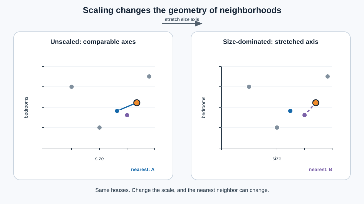
Here is where beginners get burned. The map I described depends entirely on the units you use to draw it.
Suppose you measure house size in square feet (values in the thousands) and number of bedrooms (values from 1 to 5). Now compute the distance between two houses. The size difference will dominate the bedroom difference by several orders of magnitude. Two houses that are nearly identical in size but differ by three bedrooms will look extremely close. Two houses that differ by 1,000 square feet but have the same bedroom count will look far apart.
The geometry has not changed. You have stretched one axis.
This is not a cosmetic issue. It silently rewrites which points count as neighbors. A KNN model might call a 2,000-square-foot, 2-bedroom house a near neighbor of a 2,100-square-foot, 5-bedroom house, simply because the size axis is so stretched that bedrooms barely register.
The fix is feature scaling—bringing all axes onto comparable ranges before measuring distance. Standardization and min-max scaling are the common tools. The full treatment of when and how to scale deserves its own article, but the geometric intuition is what you need here: scaling changes the shape of the map, and the shape of the map changes what the model can learn.
There are two distinct reasons to scale, and keeping them separate will save you confusion:
- Distance-based methods (KNN, k-means, SVM) measure neighborhoods directly. If one axis is stretched, "near" is decided by that axis alone.
- Linear models do not measure pairwise distance, but they combine features through weighted sums. When features have wildly different units, the coefficients become unit-sensitive, and regularization can penalize them unevenly.
Tree-based models are the notable exception. They split on single features one at a time, so scaling one axis does not change their behavior.
Common mistake: Assuming scaling is only about distance. Linear models need it too—but for a different reason. Name the mechanism before you scale.
Knowledge check
Check your understanding
Answer this question before you continue.
More Features, More Dimensions, More Trouble
Adding features sounds like adding information. Geometrically, it is adding dimensions—and dimensions are hungry.
Picture ten points scattered on a line. They are easy to tell apart. Now place the same ten points on a flat plane. They spread out a bit, but they still cluster. Now place them in a ten-dimensional space. The volume of that space grows exponentially with each new dimension, and ten points are suddenly lost in an enormous emptiness.
This is the curse of dimensionality. As dimensions grow, points spread thinner, and distances between any two points start to look alike. When every point is roughly the same distance from every other point, "near" stops meaning anything. Nearest-neighbor reasoning weakens. Clusters dissolve. The map becomes mostly empty space with a few lonely dots.
This is the geometric reason behind practical advice you will hear constantly: keep feature counts reasonable, and reduce dimensions when features multiply.
PCA is the classic response. Conceptually, PCA looks at your point cloud and finds the few directions along which the data spreads out the most. Those directions—the principal components—let you project the cloud onto fewer dimensions while keeping most of its shape.
One boundary worth knowing: PCA chooses directions of input variation without looking at your target. High variance is not guaranteed to be the most useful predictive signal. A direction with modest spread might be exactly what separates your classes. Treat PCA as a lossy projection whose usefulness must be checked against the model's actual performance.
The intuition to keep: empty space grows faster than data can fill it. More features only help if you have enough data to populate the extra dimensions.
Knowledge check
Check your understanding
Answer this question before you continue.
When the Geometry Mental Model Helps—and When It Breaks
The geometric view is durable for a specific family of models. KNN, clustering, SVM, linear models, and PCA all reason through distances, directions, boundaries, or projections in feature space. For these, picturing your data as a point cloud is not an analogy—it is literally what the algorithm computes.
But the model breaks down in two places.
First, tree-based models do not think this way. A decision tree or random forest splits on single features one at a time: "is size above 1,800 square feet?" It never measures diagonal distance across multiple features. The geometric map is the wrong picture for these models. They are more like a sequence of yes/no questions than a reading of spatial relationships.
Second, geometry still applies to categorical features—but the meaning of distance depends entirely on how you encode them. One-hot encoding places categories at the corners of a space where straight-line distance between any two categories is identical. That is a very different map from the one continuous features create. The right question is not "are my features categorical?" but "does my encoding give coordinate differences that mean what I think they mean?"
Here is when I lean on geometric intuition, and when I do not:
- Use it when choosing between KNN and linear models, when deciding whether to scale, when debugging why a distance-based model performs poorly, and when explaining PCA.
- Set it aside when working with tree ensembles, or when the dataset is so high-dimensional that "near" has already lost meaning.
The Habit Worth Building
Before you train any distance-based or linear model, run a quick mental checklist. Picture your data as a point cloud. Ask whether your axes are on comparable scales—if not, scale them. Ask whether your feature count is so high that points have spread too thin for "near" to mean anything. If so, first ask whether some features are irrelevant or redundant—those can often be dropped. Only then consider whether a projection like PCA preserves what your model needs.
Then make it physical. Take a small two-feature dataset, plot it, and before running any model, predict which points a KNN would call neighbors. Now scale one axis dramatically—say, multiply one feature by 1,000—and predict again. Watch the neighbor set change. That single exercise will teach you more about feature space than any amount of reading.
The spreadsheet view makes machine learning look like bookkeeping. The geometric view makes it what it actually is: a way of reading the shape of your data. Once you see the map, the algorithms stop being a list of names and start being a set of questions you can ask about points in space.
Knowledge check
Final check
Finish the article by checking the ideas you just learned.
References
Research updated Sep 8, 2026


