
Detect Input Distribution Shift With a Controlled Python Experiment
Your model is live. Labels arrive in three weeks. Right now, the only thing you can actually see is the input stream — and it looks different from what you…

Key topics
Your model is live. Labels arrive in three weeks. Right now, the only thing you can actually see is the input stream — and it looks different from what you trained on.
That difference is worth investigating. It is not proof your model is broken. A distribution check can tell you the inputs moved; it cannot tell you the model is now worse. Those are two different claims, and confusing them leads to blind retraining, wasted label budget, and false confidence in the other direction.
So we are going to build the smallest experiment that makes that boundary visible. We will generate data where we know exactly what changed, run three transparent diagnostics, and then deliberately break the experiment in a way the diagnostics cannot see.
What an Unlabeled Shift Check Can and Cannot Prove
Before any code, fix the epistemic boundary.
Covariate shift means the input distribution p(x) moved while the relationship p(y|x) stayed the same. Concept shift means p(y|x) moved. Label shift means p(y) moved. Only the first is directly observable without labels — you can compare inputs, but you cannot compare a relationship you cannot measure.
A detected input change is evidence of a changed world, not proof of model harm. A model can absorb mild covariate shift and still be fine. It can also fail under covariate shift it never sees. The diagnostic tells you where to look, not what you will find.
Note: Prediction-distribution monitoring is a proxy, not a measurement. It conflates input change, label change, and model behavior into one signal.
If the taxonomy itself is still fuzzy, the mental model of covariate, label, and concept shift is the prerequisite. Here we assume it and move straight to the experiment.
Set Up a Reproducible Shifted-Data Scenario
We need data where the ground truth is known, so every diagnostic can be checked against reality. The trick is to build the shift into the generator itself, not to patch it in afterward.
import numpy as np
import pandas as pd
from sklearn.model_selection import train_test_split
from sklearn.linear_model import LogisticRegression
from sklearn.metrics import roc_auc_score
from scipy.stats import ks_2samp

rng = np.random.default_rng(42)

def make_window(n, mean_shift, rng):
    # Two informative features drive the label through a fixed rule.
    f0 = rng.normal(0.0 + mean_shift[0], 1.0, n)
    f1 = rng.normal(0.0 + mean_shift[1], 1.0, n)
    # Four noise features carry no signal.
    noise = rng.normal(0.0, 1.0, (n, 4))
    # Same p(y|x) in both windows: the logit is a fixed function of f0 and f1.
    logit = 1.2 * f0 - 0.9 * f1
    p = 1.0 / (1.0 + np.exp(-logit))
    y = rng.binomial(1, p)
    cols = [f"f{i}" for i in range(6)]
    X = np.column_stack([f0, f1, noise])
    return pd.DataFrame(X, columns=cols).assign(target=y)

train = make_window(3600, mean_shift=(0.0, 0.0), rng=rng)
later = make_window(2400, mean_shift=(1.5, -1.0), rng=rng)
cols = [f"f{i}" for i in range(6)]
Environment assumptions: Python 3.9+, NumPy, pandas, scikit-learn, SciPy. No external services, no credentials, no network access. Everything is deterministic under the seeded generator.
Why synthetic? Because we built the shift into the input means of f0 and f1 while keeping the label rule logit = 1.2*f0 - 0.9*f1 identical in both windows. That is a genuine covariate shift: p(x) moved, p(y|x) did not. When a diagnostic fires, we can confirm it found the thing we planted. On real data, you never get that check.
Common mistake: Shifting feature values after the labels are drawn changes p(y|x) too, because the same labels now sit on different inputs. If you patch the data instead of the generator, you have quietly created concept shift and your "covariate" experiment is lying to you.
Knowledge check
Check your understanding
Answer this question before you continue.
Diagnostic 1: Compare Per-Feature Distributions
The cheapest check is a table of summary statistics per feature.
summary = pd.DataFrame({
    "train_mean": train[cols].mean(),
    "later_mean": later[cols].mean(),
    "train_std": train[cols].std(),
    "later_std": later[cols].std(),
})
summary["mean_delta"] = summary["later_mean"] - summary["train_mean"]
print(summary.round(3))
Expected output: f0 and f1 show large mean_delta values (roughly +1.5 and -1.0). The other four features sit near zero.
For a per-feature signal with a test statistic, use the Kolmogorov–Smirnov two-sample test:
for c in cols:
    stat, p = ks_2samp(train[c], later[c])
    print(f"{c}: KS={stat:.3f}  p={p:.2e}")
The shifted features light up with small p-values; the untouched features stay quiet. That is the success criterion — the diagnostic found what we planted.
Common mistake: With many features, some tests will flag by chance. A p-value is a candidate for investigation, not a verdict. Treat flags as a queue, not a conclusion.
Knowledge check
Check your understanding
Answer this question before you continue.
Diagnostic 2: Adversarial Validation
Per-feature tests miss shifts spread across many features jointly. Adversarial validation catches them.
Label every row as 0 (training) or 1 (later), train a classifier to separate the two windows, and read the AUC as a shift score.
adv = pd.concat([train[cols], later[cols]], ignore_index=True)
adv["is_later"] = [0]*len(train) + [1]*len(later)

Xa = adv[cols].values
ya = adv["is_later"].values
Xa_tr, Xa_te, ya_tr, ya_te = train_test_split(Xa, ya, test_size=0.3, random_state=0)

clf = LogisticRegression(max_iter=1000).fit(Xa_tr, ya_tr)
auc = roc_auc_score(ya_te, clf.predict_proba(Xa_te)[:, 1])
print(f"Adversarial AUC: {auc:.3f}")
Interpretation: AUC near 0.5 means the windows are indistinguishable. AUC well above 0.5 means the inputs are separable — something moved. Here you should see a high AUC, driven by f0 and f1.
Inspect clf.coef_ before concluding. A high AUC can come from a few dominant features or from a genuinely different sampling process. The score tells you that the windows differ; the coefficients hint at where.
Knowledge check
Check your understanding
Answer this question before you continue.
Diagnostic 3: Watch the Prediction Distribution
This is the only label-free signal that touches the model itself.
model = LogisticRegression(max_iter=1000).fit(train[cols], train["target"])

train_scores = model.predict_proba(train[cols])[:, 1]
later_scores = model.predict_proba(later[cols])[:, 1]

print(f"train positive rate: {(train_scores > 0.5).mean():.3f}")
print(f"later positive rate: {(later_scores > 0.5).mean():.3f}")
A large shift in predicted-positive rate is a useful alarm. But it conflates input change, label change, and model behavior. It is a trigger, not a diagnosis.
The combination matters. Input shift with a stable prediction rate is a different situation than input shift with a collapsing prediction distribution. But read that carefully: a stable aggregate rate only says the share of positive predictions did not move. It does not say the predictions are still correct. Errors can shift underneath a flat rate — the model can be wrong on a different set of rows while the total count of positives stays put. Stable output is not evidence of robustness; it is evidence that this one coarse signal stayed quiet.
Warning: A poorly calibrated model produces misleading prediction distributions. If your scores were never trustworthy, do not read meaning into their movement.
What the Experiment Proves — and What It Does Not
Map each diagnostic back to what we injected:
| Diagnostic | What it measures | What it found here |
|---|---|---|
| Per-feature stats + KS | Marginal p(x) per feature | f0, f1 shifted |
| Adversarial validation | Joint p(x) separability | High AUC |
| Prediction distribution | Model output under new inputs | Possible rate shift |
The input-side checks fired because we changed p(x). The concept relationship p(y|x) was never touched, so no diagnostic can claim concept drift — and none should.
Here is the hard limit, stated plainly: none of these diagnostics can confirm concept drift or quantify performance loss without delayed labels. They are covariate-shift detectors. Naming them correctly is what prevents false confidence.
Decision rule: treat a shift signal as a reason to investigate and prioritize label collection, not as a reason to retrain blindly.
Modify the Experiment: Add Concept Shift and See What Breaks
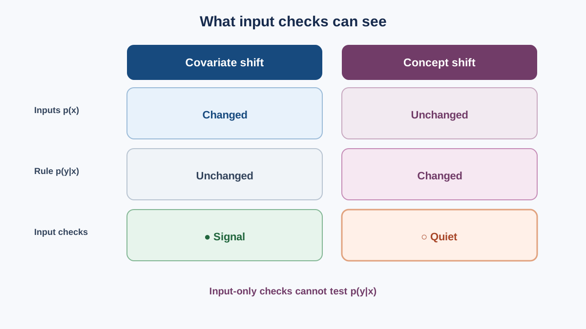
Now the important part. Change the experiment so p(y|x) shifts while p(x) stays fixed.
later_concept = later.copy()
# Flip labels for rows where f2 is above its median — a pure concept change.
mask = later_concept["f2"] > later_concept["f2"].median()
later_concept.loc[mask, "target"] = 1 - later_concept.loc[mask, "target"]
Rerun all three diagnostics against later_concept. The input-side checks report nothing — because p(x) is identical. Only the prediction distribution may wobble, and even that is unreliable.
This is the most important takeaway in the article. The tools you built are covariate-shift detectors. They are blind to the shift that most directly damages model performance. If you call them "drift detectors" without qualification, you will trust them in exactly the case where they cannot help.
The follow-up is a delayed-label evaluation step: once labels arrive, measure actual performance on the later window and close the loop. That measurement — not the input diagnostic — is what tells you whether the model is still healthy.
Knowledge check
Check your understanding
Answer this question before you continue.
Where to Go From Here
Run input-side diagnostics continuously. They are cheap, label-free, and they catch real changes early. But treat every signal as a question, not an answer.
The practical loop: monitor inputs for covariate shift, monitor predictions as a secondary alarm, and pair both with a delayed-label evaluation so the model's actual health is eventually measured rather than inferred. The diagnostics tell you where to look. Only labels tell you what you found.
Your next step: take this experiment and replace the synthetic data with a slice of your own training data and a recent batch of production inputs. Run the same three diagnostics. You will not have ground truth — which is exactly why building the controlled version first was worth the hour.
Knowledge check
Final check
Finish the article by checking the ideas you just learned.
References
Build stronger machine learning foundations
Use structured resources to connect theory, scikit-learn workflows, and evaluation practice.


