Covariate, Label, and Concept Shift: Formal Definitions and Limits

A model degrades in production. Three engineers offer three diagnoses: "the inputs drifted," "the class balance changed," "the meaning changed." All three sound reasonable, and each one points to a different fix. The trouble is that these names usually get used as vibes rather than equations, so nobody can say precisely what moved.

This article pins each claim to a specific distribution. Once you can write down which factor of the joint distribution changed, you can state exactly what you are allowed to assume — and what that assumption quietly forbids.

If you have already built the intuition that the world changes after training, this is the formal follow-up. We stop describing shift and start defining it.

One Joint Distribution, Three Ways to Break It

Everything here lives inside one object: the joint distribution $p(x, y)$. It fully describes the data-generating process — which feature vectors appear, and which labels come with them.

You can factor that joint two ways, and both are algebraically equivalent:

$p(x, y) = p(x) \cdot p(y \mid x)$

$p(x, y) = p(y) \cdot p(x \mid y)$

The pieces have names worth fixing in your head:

• $p(x)$ — the covariate (feature) marginal. Which inputs show up.
• $p(y)$ — the label marginal. How often each class appears.
• $p(y \mid x)$ — the conditional that maps features to labels.
• $p(x \mid y)$ — the conditional that describes what each class looks like.

Now introduce two worlds. The source distribution $p_s$ is what you trained on. The target distribution $p_t$ is what you deploy into. Distribution shift simply means $p_s(x, y) \neq p_t(x, y)$.

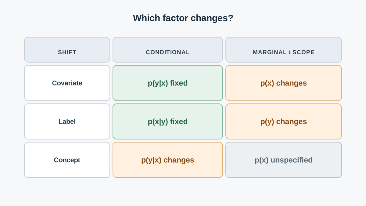
Here is the structural point that makes the three names non-interchangeable: the two factorizations are equivalent, but each shift definition freezes a different factor. Covariate shift freezes $p(y \mid x)$. Label shift freezes $p(x \mid y)$. Concept shift breaks a conditional outright. Same joint, three different bets about which part stayed still.

Covariate Shift: Inputs Move, the Rule Holds

Definition. Covariate shift holds when

$p_s(x) \neq p_t(x) \quad \text{while} \quad p_s(y \mid x) = p_t(y \mid x).$

The mapping from features to labels is stable. Only the region of feature space you are visiting has changed.

That conditional-equality clause is the whole point. It is the license that lets you reweight source samples to look like target samples. Watch the algebra fall out. You want the target risk:

$R_t = \mathbb{E}_{p_t}\big[L(y, f(x))\big] = \int L(y, f(x))\, p_t(x, y)\, dx\, dy.$

Factor the target joint as $p_t(x)\, p_t(y \mid x)$, then multiply and divide by the source marginal $p_s(x)$:

$R_t = \int L(y, f(x))\, p_t(y \mid x)\, \frac{p_t(x)}{p_s(x)}\, p_s(x)\, dx\, dy.$

Because covariate shift guarantees $p_t(y \mid x) = p_s(y \mid x)$, the first two factors collapse back into the source joint:

$R_t = \mathbb{E}_{p_s}\!\left[\frac{p_t(x)}{p_s(x)}\, L(y, f(x))\right].$

The weight $w(x) = p_t(x) / p_s(x)$ falls straight out of the algebra. Samples that look more like the target get more say; samples that look less like it get less. That is the entire mechanism behind importance weighting.

The support condition. That identity only holds where the source distribution actually puts mass. If some target inputs live in a region where $p_s(x) = 0$, the ratio $p_t(x)/p_s(x)$ is undefined there, and no amount of reweighting source examples can estimate target risk in that region — you have no source data to weight. This is the support-overlap requirement, and it is the first thing to check before trusting any importance-weight correction. Regions that appear only in the target are not a weighting problem; they are a data problem.

Limits. The assumption says nothing about whether your model class can actually fit the stable conditional — a stable rule you cannot represent is still a rule you will miss. And it fails the moment the conditional itself moves.

Example. A spam filter trained on one year of mail, deployed on a year where certain vocabulary became common. Same spam-versus-not-spam rule, different feature mix. Reweighting the old mail toward the new vocabulary distribution is defensible here — provided the new vocabulary still appears in the old data.

Label Shift: The Balance Moves, the Class Signature Holds

Definition. Label shift holds when

$p_s(y) \neq p_t(y) \quad \text{while} \quad p_s(x \mid y) = p_t(x \mid y).$

Each class still looks the way it always looked. Only how often each class appears has changed. This is sometimes called prior probability shift, and the name is honest about what moved.

Choosing it. Label shift is a reasonable bet when $y$ causes $x$: a disease produces symptoms, so the symptoms given the disease stay stable while prevalence changes. Covariate shift is a reasonable bet when $x$ causes $y$, or when the label is assigned from the features. Treat causal direction as motivation for a candidate assumption, not proof of it. A plausible causal story does not establish that the relevant conditional actually stayed stable — only labeled target data can settle that.

The correction. For a sample with label $y$, the factor is $p_t(y) / p_s(y)$. Notice this is a per-class weight, not a per-sample one — every example of the same class gets the same multiplier. The derivation mirrors the covariate case, but the ratio lives on the label marginal instead of the feature marginal.

The practical catch. You do not observe $p_t(y)$ directly; you only have unlabeled target data. Estimating it typically means running your classifier on that data and inverting a confusion matrix. That estimate is circular if the model is already bad — you are using the thing under suspicion to diagnose itself.

Example. A classifier trained on a balanced dataset, deployed where the positive class is rare. Same class-conditional feature distributions, different prevalence.

Concept Shift: The Rule Itself Changes

Definition. Concept shift holds when

$p_s(y \mid x) \neq p_t(y \mid x).$

The conditional relationship between features and labels is no longer the same function.

Contrast this with the other two. Covariate and label shift each preserve a conditional and move a marginal. Concept shift breaks the conditional itself. That difference is not cosmetic — it is the difference between a problem you can correct with the data you already have and one you cannot.

The precise limit. The definition says only that $p(y \mid x)$ changed. It does not say that $p(x)$ stayed fixed, and it does not say the new relationship is unlearnable. What it does say is narrower and more useful: from source labels alone — or from source labels plus unlabeled target inputs — the new conditional is not identifiable. The old labels describe a rule that no longer holds, so no reweighting of them can reconstruct the new one. But if you can obtain labeled target data, or bring in additional structural assumptions, adaptation is possible. Concept shift is a limit on what your existing data can tell you, not a proof that the problem is hopeless.

A terminology trap. "Concept drift" gets used loosely for any degradation over time, including pure covariate shift. Insist on the conditional-distribution test before accepting the label. If $p(y \mid x)$ is intact, you have a reweighting problem, not a concept problem.

Example. A fraud model where a previously benign transaction pattern became the signature of fraud. Same features, inverted meaning. Relabeling or retraining on fresh target data is the honest response; reweighting the old labels is not.

What Each Definition Does and Does Not Justify

Shift type	Frozen factor	Moving factor	Correction licensed	What the assumption fails to guarantee
Covariate	$p(y \mid x)$	$p(x)$	Importance weights $p_t(x)/p_s(x)$, where support overlaps	That target inputs lie inside source support; that your model class can fit the stable rule
Label	$p(x \mid y)$	$p(y)$	Per-class weights $p_t(y)/p_s(y)$	That you can estimate $p_t(y)$ without a good classifier
Concept	neither	$p(y \mid x)$	None from old labels alone	That the new conditional is unlearnable — target labels or extra assumptions can still enable adaptation

Non-identifiability. From unlabeled target data alone, you cannot tell which shift occurred. The three hypotheses can produce identical observed feature distributions, so the choice is an assumption, not a measurement. This is the single most important limit in the table.

The implication trap. Covariate shift and concept shift both generally imply a change in $p(y)$, and label shift generally implies a change in $p(x)$. So "the class balance changed" is not evidence for label shift — it is consistent with all three.

The degenerate case. When the label is a deterministic function of the features, the covariate-shift assumption is satisfied even when $y$ causes $x$. The two assumptions can hold at once, which is why the names are not mutually exclusive in every corner of the space.

The realistic case. Real deployments often violate all three clean assumptions simultaneously. Joint-shift framings exist for exactly this reason; treat that as a boundary marker, not a full treatment.

Choosing an Assumption Without Fooling Yourself

The decision rule is one question: which conditional am I willing to bet is stable, and why? Justify it from the causal direction of the problem, not from which correction method your tooling happens to support.

• Covariate shift when you can plausibly reweight inputs, the feature-to-label rule is genuinely fixed, and target inputs fall inside source support.
• Label shift when prevalence is the moving part and you trust the class signatures.
• Concept shift when you should stop correcting and start relabeling or retraining.

When not to use them. Do not apply importance weighting when the weight distribution is extreme. A few samples dominate the estimate and its variance explodes — you get a confident-looking number built from almost no effective data. And do not apply it at all when target inputs fall outside source support; there is nothing to reweight.

The common mistake. Assuming a shift type because a monitoring dashboard flagged a feature distribution change. That only establishes $p(x)$ moved. It says nothing about which assumption holds.

The practical check. Verify the frozen conditional on data you can actually label. The assumption is a bet; the labeled sample is the settlement. I would rather spend an afternoon labeling a few hundred target examples than ship a correction built on a conditional I never tested.

The three names collapse into one question you can carry into any deployment: which factor of $p(x, y)$ am I willing to assume is stable, and what does that assumption let me do? The definitions are not vocabulary to memorize. They are constraints that determine whether correction is even possible.

Pick one model you have deployed or evaluated. Write down its $p_s$ and $p_t$ factorization explicitly. Then test whether the conditional you assumed stable actually is — before you reach for a correction method.