Error Analysis in Machine Learning: Turn Bad Predictions Into Next Experiments

You improved the model twice. The validation score went up, then up again. Now every change you try makes it worse or does nothing. You are not out of ideas—you are out of information. The score is a summary, not a diagnosis.

That distinction is the whole game. An aggregate metric tells you how wrong the model is on average. It does not tell you where it is wrong, why it is wrong, or for whom. Error analysis in machine learning is the bridge between those two questions: from "how wrong am I" to "what should I change next."

The workflow is repeatable: slice, inspect, hypothesize, experiment. Each step narrows the space of possible causes until you are testing one idea at a time instead of guessing.

Why One Score Is Not a Diagnosis

A validation score averages over every example in your evaluation set. That is its strength and its trap. The average hides the structure of failure: which rows, which classes, which feature ranges.

Two models can have identical accuracy with completely different failure profiles. One fails evenly across all groups—a little wrong everywhere, like a student who guesses on every question. The other fails catastrophically on one slice—perfect on most cases, broken on a specific subgroup, like a student who aces everything except word problems. Same average. Different problems. Different fixes.

The first model might need more capacity or better features. The second model needs you to understand what makes that subgroup different. If you only watch the aggregate, you cannot tell which situation you are in.

Error analysis turns your metric into a list of testable causes. As you work through the workflow, you are trying to distinguish four candidate bottlenecks:

• Data quality: the rows are missing, noisy, or mislabeled.
• Representation: the signal exists in the world but not in your features.
• Model capacity: the model is too simple to capture the pattern.
• Decision threshold: the model ranks well but draws the line in the wrong place.

Each bottleneck has a different fix. The workflow exists to tell them apart.

Slice Your Errors Before You Judge Them

A slice is a subset of predictions that share a value or range of a feature: a class, a segment, a time window, a feature bucket. Slicing is how you make the structure of failure visible instead of averaged away.

Start with the slices you already suspect matter. The minority class in an imbalanced problem. The classes that blur together in your confusion matrix. The rows where the model is most confident and still wrong. Pick one or two features per pass—slicing on too many dimensions at once produces noise, not signal.

For each slice, compare its local error rate against the overall error rate. Suppose your model is 90% accurate overall. A slice with 95% accuracy is fine. A slice with 70% accuracy is where the model is disproportionately failing. That gap is your lead.

Here is what the same overall accuracy can hide:

Slice	Model A error rate	Model B error rate
Overall	10%	10%
New customers	9%	35%
Returning customers	11%	4%

Model A fails evenly. Model B has a returning-customer problem hiding inside a respectable average. If you deployed Model B without slicing, you would discover the failure in production, where it costs more to fix.

Common mistake: Slicing on too many dimensions at once. Two features per pass is plenty. You are looking for a pattern you can act on, not building a complete map of every interaction.

Inspect the Worst Slice, Not the Average

Now zoom in. Pull the actual rows the model got wrong in your worst slice and read them like evidence, not like a list of failures.

You are looking for what the errors share. A missing feature that the model needed. An ambiguous label that even a human would struggle to assign. A rare value that never appeared in training. A pattern the model simply never saw.

The most informative errors are the high-confidence wrong ones—rows where the model was certain and still missed. These are your highest-priority inspection targets, because the model is not hesitating near a boundary; it is confidently applying a rule that does not match reality. That makes them excellent clues. But a clue is not a conclusion. Confidence tells you the model's score was far from the cutoff—it does not tell you whether the problem is a missing feature, a wrong label, a shifted distribution, or a model that learned the wrong rule. Sort the possibilities by inspecting the rows themselves.

As you read, sort your findings into three buckets:

• Data problems: bad or missing labels, contradictory examples.
• Representation gaps: the model lacks a signal that exists in the input but is not encoded in a feature.
• Genuine difficulty: the example is ambiguous even for a human expert.

The third bucket matters more than beginners expect. Not every error is fixable. Some rows are just hard, and the model's mistakes on them are not evidence of a defect.

Warning: Do not fix one error by hand. Fix the pattern the error reveals. If you patch individual cases, you are memorizing the test set, not improving the model.

Form a Hypothesis About the Bottleneck

You have inspected the errors. Now name the bottleneck before you change anything. A named bottleneck turns your next experiment from a guess into a test.

Map your findings to the four categories:

• Data bottleneck: errors cluster on rows with missing, noisy, or contradictory labels. The model is learning from targets that lie.
• Representation bottleneck: errors share a feature the model cannot see. The signal exists in the world—in the raw input—but not in the columns you gave the model.
• Capacity bottleneck: errors are spread broadly across all slices, and your learning curves still show training and validation gap closing as you add complexity.
• Threshold bottleneck: errors concentrate near the decision boundary, and shifting the threshold changes which error type dominates.

The threshold branch deserves one extra check before you commit to it. Look at the predicted probabilities or decision scores for the affected slice, not just the final class labels. If the model ranks the slice's examples poorly—positives scoring below negatives—you have a ranking problem that threshold tuning cannot fix. If the ranking is sound but the cutoff sits at the wrong place, adjusting the threshold changes which error type dominates without retraining. That distinction is the difference between a model problem and a decision problem.

The decision rule is simple: name the bottleneck before you change anything. If you cannot name it, you have not finished inspecting. If you name it, you know what to test.

This is where error analysis connects to the broader diagnostic toolkit. Learning curves help confirm a capacity hypothesis. Bias-variance reasoning distinguishes underfitting from overfitting. Threshold analysis tells you whether the model's ranking is sound and the cutoff is wrong. You do not need to re-learn those tools here—you need to know which one your hypothesis calls for.

Run One Targeted Experiment

Each bottleneck suggests a different next move:

Bottleneck	Targeted experiment
Data quality	Clean or relabel the worst slice, then retrain
Representation	Engineer a feature that captures the missing signal
Model capacity	Increase complexity or add relevant data
Decision threshold	Adjust the cutoff using the cost of each error type

Change one thing at a time. A combined change cannot be attributed—if you add a feature and clean labels in the same run, you will not know which one moved the score.

After the experiment, re-run your error analysis on the same slice. The question is not "did the overall score go up?" It is "did the slice I targeted actually improve?" A small bump in the aggregate can hide a worst slice that barely moved. The goal is to fix the diagnosed failure, not to chase the average.

Common mistake: Celebrating an overall-score improvement when the slice you diagnosed is still broken. The aggregate can improve for reasons unrelated to your hypothesis—and your real problem can remain untouched.

When Error Analysis Misleads You

The workflow is powerful, but it has failure modes. Know them before you trust your slices.

Small slices produce noisy error rates. A 50% error rate on five examples is not evidence of anything. Always check the slice size before you draw conclusions. If you cannot act on the slice because it is too small to matter, move on.

The worst rate is not always the highest priority. A slice with a terrible error rate but only a handful of examples may matter less than a slice with a moderate error rate that covers thousands of predictions. Rank candidate slices by three things together: local error rate, the share of total errors the slice contains, and the real-world cost of getting that slice wrong. The slice your users feel is the slice that deserves your next experiment.

Slicing on easy dimensions can hide the real problem. Slice on the dimensions that matter to your deployment—the segments your users care about, the conditions your model will face—not just the features that are convenient to group by.

Correlation is not cause. A slice with high error may share a feature that is merely correlated with the true cause. The shared feature is a clue, not a conclusion. Your experiment is what tests the causal claim.

Error analysis on a broken evaluation setup sends you chasing phantoms. If your validation set leaks training information or is mis-split, the error patterns you find are artifacts. Confirm your evaluation setup before you trust any slice.

And know when to stop. Error analysis is iterative, not infinite. Set a stopping rule based on the cost of the remaining errors. If the worst slice you can find is small, noisy, or genuinely difficult, further analysis has diminishing returns. Ship the model, monitor it in production, and let real-world data tell you where the next slice lives.

The Loop, Not the Cleanup

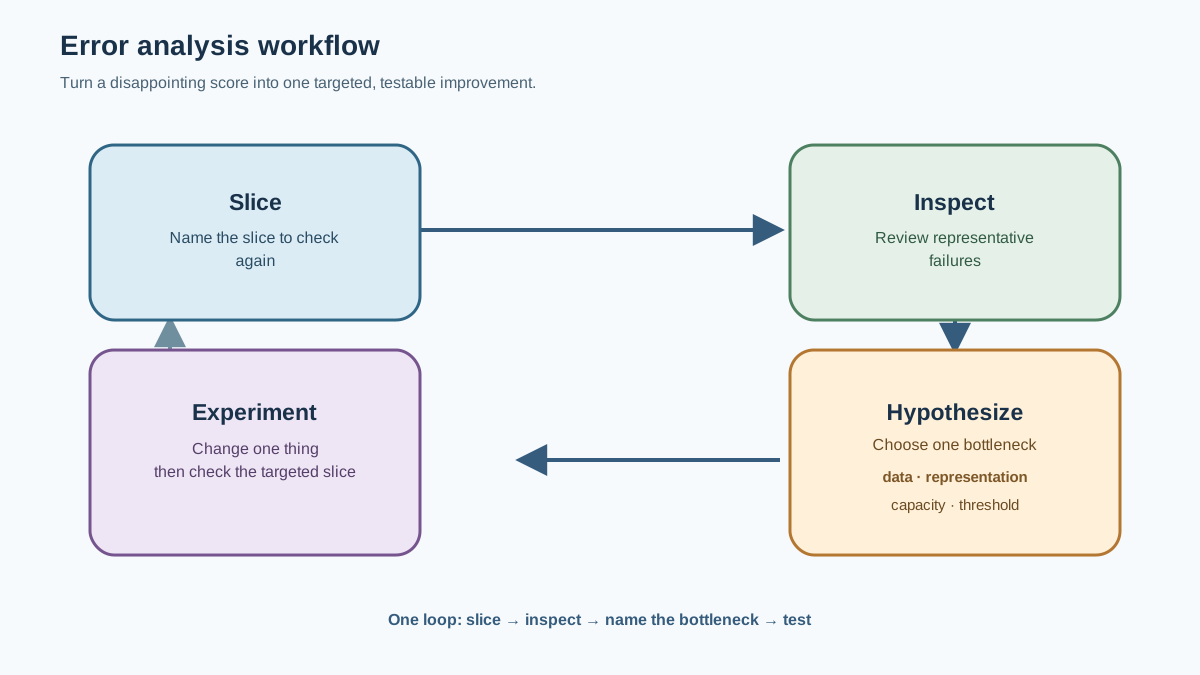
Error analysis is not a one-time cleanup you perform after training. It is a loop you run whenever the model disappoints you: slice, inspect, hypothesize, experiment. Each pass should leave you with one named bottleneck and one test of it.

Here is your next step. Take the model you already have. Pick the slice where it fails most. Pull five of its errors and read them—five examples are an inspection start, not proof of a pattern, so treat them as leads to verify rather than conclusions. Name the bottleneck—data, representation, capacity, or threshold—before you change a single line of code.

The score told you the model was wrong. The slice tells you where. The inspection tells you why. The experiment tells you whether you were right. That is the difference between reacting to a number and debugging a system.

References

Research updated Sep 8, 2026