Simulate Label Shift and Test Prior-Probability Correction

Your model passed validation. Then it went to production and started predicting one class far more often than it should. The features look normal. The model file hasn't changed. So what broke?

Usually, nothing broke. The world changed the mix of classes, not the shape of the classes. That specific change has a name — label shift — and it has a specific repair. In this tutorial we'll build a controlled simulation where we know the true answer, watch the model fail, apply the correction, and then break the assumption on purpose to see exactly where the repair stops working.

What Label Shift Actually Changes

Before any code, get the assumption precise, because the whole experiment is a test of one claim.

Label shift means the label marginal p(y) changes while the class-conditional distribution p(x|y) stays fixed. The features that belong to each class look the same; only the proportion of each class changes.

That is the opposite of covariate shift, where p(x) changes but p(y|x) stays fixed. If you've read the distribution-shift overview, you already have the taxonomy. Here we only need the one boundary that makes this experiment meaningful: under label shift, the stable object is the class-conditional distribution, not the input distribution.

Why would that ever be the right assumption? Because label shift fits anticausal problems, where the label causes the features. A disease causes symptoms. A fraud pattern causes transaction features. When the prevalence of the disease rises — a pandemic, a seasonal outbreak — the symptoms each disease produces don't change. Only how often each disease appears changes.

And here is the part that trips people up: the optimal decision rule can change even when the model is unchanged. The posterior p(y|x) depends on the prior p(y). If the prior moves, the correct answer for a given input moves with it. Your model is still doing its job; it's answering a question about the old world.

For the correction to be valid, two assumptions have to hold:

• Every class has nonzero support in the source data. You cannot recover a class you never saw.
• The confusion matrix of your predictor is invertible. We'll see why in a moment, and what happens when it isn't.

Set Up the Controlled Simulation

The reason to start synthetic is simple: you cannot diagnose a correction method on data where you don't know the true prevalence. Here, we do.

You need Python with NumPy, pandas, and scikit-learn. No credentials, no external services.

import numpy as np
import pandas as pd
from sklearn.linear_model import LogisticRegression

rng = np.random.default_rng(0)

# Fixed class-conditional distributions: p(x|y) never changes.
# Class 0: mean [-1, -1]; Class 1: mean [1, 1]. Same covariance.
def sample_class(n, mean):
    return rng.normal(loc=mean, scale=1.0, size=(n, 2))

def make_set(n, prevalence):
    n1 = int(round(n * prevalence))
    n0 = n - n1
    X = np.vstack([sample_class(n0, [-1, -1]),
                   sample_class(n1, [ 1,  1])])
    y = np.array([0] * n0 + [1] * n1)
    return X, y

# Source: 50/50. Target: 90/10 — the minority class got rare.
X_src, y_src = make_set(4000, prevalence=0.5)
X_tgt, y_tgt = make_set(4000, prevalence=0.1)

clf = LogisticRegression().fit(X_src, y_src)
p_src = clf.predict_proba(X_src)[:, 1]
p_tgt = clf.predict_proba(X_tgt)[:, 1]

The class-conditional distributions are identical by construction — same means, same scale — while the label marginals differ. That is the whole point of the setup. If you plot the two feature clouds per class, they overlap. If you count labels, they don't.

Watch the Model Fail Without Changing

Now measure the failure before you try to fix it.

def predicted_freq(p, thr=0.5):
    return (p >= thr).mean()

print("source predicted positive rate:", predicted_freq(p_src))
print("target predicted positive rate:", predicted_freq(p_tgt))
print("target true positive rate:     ", y_tgt.mean())

The model predicts roughly the source prevalence on the target set, not the target prevalence. It is tracking the old world.

Here's the trap: ranking quality can stay nearly flat while the thresholded decisions degrade. Compute ROC AUC on the target set and you'll find it barely moved. The model still orders examples correctly. It just places the threshold in the wrong spot for this prevalence.

So accuracy alone will lie to you. The metric that exposes the problem is minority-class recall or precision — or a calibration check. Under a 90/10 target, a model tuned for 50/50 will under-call the minority class and over-call the majority.

Common mistake: Treating this as overfitting or a broken model. It is neither. It is a prior mismatch, and it is invisible if you only ever evaluate on source-like data.

A useful diagnostic is a side-by-side histogram of predicted probabilities for source and target, with the decision threshold drawn in. You'll see the target mass shift left of the threshold.

Estimate the Target Prevalence

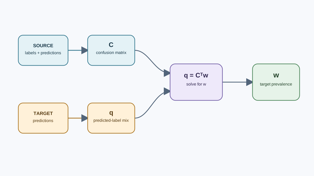
Now the correction. The mechanism is a moment-matching identity, and it's worth understanding rather than memorizing.

Let C be the confusion matrix of your predictor on source data, where entry C[i, j] is the probability the model predicts class j when the true class is i. Let q be the vector of predicted-label frequencies on the unlabeled target set. Let w be the unknown target prevalence vector. The identity is:

q = Cᵀ w

So you can recover the target prevalence by inverting the confusion matrix:

w = (Cᵀ)⁻¹ q

Each symbol maps to a column in your DataFrame: C comes from source predictions versus source labels, q comes from target predictions alone, and w is what you're solving for. This is the core of Black Box Shift Estimation.

from sklearn.metrics import confusion_matrix

# Confusion matrix on source: rows = true, cols = predicted.
C = confusion_matrix(y_src, (p_src >= 0.5).astype(int), normalize="true")

# Predicted-label frequencies on target (unlabeled in practice).
q = np.array([(p_tgt < 0.5).mean(), (p_tgt >= 0.5).mean()])

w_hat = np.linalg.solve(C.T, q)
print("estimated target prevalence:", w_hat)
print("true target prevalence:     ", [0.9, 0.1])

Two practical warnings. First, the confusion matrix must be invertible; if two classes are indistinguishable to the model, the matrix is singular and the solve fails or explodes. Second, the estimate can come out negative or above one. That is not a bug in your arithmetic — it is a signal that an assumption is violated.

Note: Moment matching is one approach. Maximum-likelihood estimation of the label marginal often performs better in practice, so don't treat this as the only tool in the box.

Apply the Prior Correction and Re-Measure

With the estimated prevalence, adjust the predicted probabilities by the ratio of target to source prevalence, then renormalize.

src_prev = np.array([0.5, 0.5])
ratio = w_hat / src_prev

# Reweight the two-class probabilities, then renormalize.
probs = clf.predict_proba(X_tgt)
adjusted = probs * ratio
adjusted /= adjusted.sum(axis=1, keepdims=True)
p_adj = adjusted[:, 1]

print("adjusted predicted positive rate:", predicted_freq(p_adj))

Re-evaluate with the same metrics you used before the correction, so the comparison is honest. What you should see: predicted class frequencies move toward the true target prevalence, and the corrected probabilities better reflect the target prior. But do not expect every metric to improve. The correction shifts the positive decision boundary against the minority class, so positive calls generally become less frequent. Precision and recall move in opposite directions depending on where the threshold sits, and neither is guaranteed to improve.

That last point matters. The correction changes decisions, not the ranking. It shifts the operating point; it does not make the model smarter. If your ranking was bad, reweighting won't rescue it.

Your success criterion: the estimated prevalence lands within a stated tolerance of the known true target prevalence on this simulated data. A reasonable tolerance for this setup is 0.03 absolute error on each class. If your estimate falls outside that band, check the confusion matrix conditioning and the target sample size before trusting the correction.

Where the Correction Breaks

This is the section I'd read twice, because the failure modes are quiet.

If the true shift is covariate shift or concept drift, the correction will silently produce confident nonsense. The estimator assumes p(x|y) is fixed. Feed it a world where that's false and it will still return a number — a wrong one.

Small target samples make the prevalence estimate noisy. Rerun the simulation across several random seeds and watch the estimate jitter. With a few hundred target examples, the variance alone can swamp the signal.

Classes absent from the source data cannot be recovered by any reweighting scheme. There is no weight for a class you never trained on.

A near-singular confusion matrix amplifies estimation error. Check the condition number of C before trusting the output.

Decision rule: Use prior correction only when you have a defensible reason to believe the class-conditional distributions are stable, and validate the estimate against any labeled target data you can obtain.

One Follow-Up Experiment

The fastest way to internalize the boundary is to violate it on purpose.

Change the simulation so the class-conditional means also shift — move the target class means by a full unit — then rerun the same pipeline. The prevalence estimate degrades, and the corrected decisions get worse, not better. The method is only as good as its assumption.

A second variation: sweep the severity of the prevalence change and plot estimation error against shift magnitude. That turns this tutorial into a reusable diagnostic harness you can point at your own data.

The Takeaway

Prior correction is a targeted repair for one specific assumption, not a general fix for distribution shift. Before you reach for it, verify that p(x|y) is plausibly stable. Then estimate prevalence. Then confirm the estimate against any labeled target data you can get your hands on before you trust adjusted decisions.

The next practical step is small and worth building: a monitoring check that compares predicted class frequencies against expected prevalence over time. When those two lines diverge, you'll know the world moved before your metrics do.