
Compare Raw and Calibrated Probabilities With Scikit-Learn
A model can rank every sample correctly and still lie about the number attached to each one. This experiment isolates that lie, then measures whether a…

Key topics
A model can rank every sample correctly and still lie about the number attached to each one. This experiment isolates that lie, then measures whether a calibration step repairs it.
You already know how to read a classifier score. Now you want to know whether that score means what it says. If the model prints 0.8, do roughly 80% of those samples actually belong to the positive class? That is the calibration question, and it is separate from whether the model sorts positives above negatives.
This tutorial runs a controlled experiment: one base model, one fixed set of scores, and a calibration step applied on top. We fit a classifier, read its raw probabilities, fit a calibrator on data the base model never saw, and compare both on a test set neither one touched. The success criterion is stated up front so you know what a win looks like before you write a line of code.
What This Experiment Will Prove
The question is narrow: does a calibration step make predicted probabilities more trustworthy on unseen data?
Two signals answer it:
- A reliability diagram that sits closer to the diagonal.
- A lower Brier score on held-out data.
If neither improves, calibration did not help this model on this data, and that is a real result worth knowing.
Two boundaries keep the experiment honest. First, calibration is a monotonic remapping of scores. When you apply a calibrator to a fixed model's outputs, the order of samples is preserved — so AUC-style ranking metrics should stay essentially flat. (Isotonic regression can create ties by mapping several distinct scores to the same value, which nudges ranking metrics slightly.) Second, calibration is not threshold selection. Moving the decision threshold changes which samples you call positive; it does not change whether the scores are reliable. Those are different jobs.
Note: If reliability diagrams and the calibration-versus-ranking distinction are still fuzzy, read the calibration concept article first. This piece assumes that mental model and spends its words on the experiment.
Knowledge check
Check your understanding
Answer this question before you continue.
Setup, Data, and the Honesty Rule
You need Python with scikit-learn, NumPy, pandas, and matplotlib. No external services, no credentials.
Use a dataset with enough samples and a non-trivial positive rate so reliability bins are not empty. A synthetic set from make_classification works well because you control the size and balance.
import numpy as np
from sklearn.datasets import make_classification
from sklearn.model_selection import train_test_split

X, y = make_classification(
    n_samples=8000,
    n_features=20,
    n_informative=10,
    n_redundant=2,
    weights=[0.7, 0.3],
    flip_y=0.05,
    random_state=42,
)

X_train, X_test, y_train, y_test = train_test_split(
    X, y, test_size=0.3, stratify=y, random_state=42
)

print("train:", X_train.shape, "test:", X_test.shape)
print("positive rate:", y.mean().round(3))
Expected output looks like this:
train: (5600, 20) test: (2400, 20)
positive rate: 0.301
Now the rule that makes the whole experiment valid: the calibrator must never see the rows used to fit the base classifier. Fit a calibrator on its own training rows and you get optimistic, meaningless calibration. The calibrator learns to map scores it has already memorized.
The cleanest design reserves three disjoint splits: a model-training split to fit the base classifier, a calibration split to fit the calibrator on that fixed model's scores, and a test split for the final comparison. The base model is fit once and never refit. That is what makes the comparison controlled — the only thing that changes between raw and calibrated is the mapping applied to the same scores.
Knowledge check
Check your understanding
Answer this question before you continue.
Fit the Base Classifier and Read Its Raw Probabilities
Pick a base model with a known calibration tendency. Maximum-margin and tree-based models are good teaching choices because their scores get pushed toward the extremes — they rarely say "maybe."
from sklearn.ensemble import RandomForestClassifier
from sklearn.metrics import brier_score_loss

base = RandomForestClassifier(n_estimators=300, random_state=42)
base.fit(X_train, y_train)

raw_proba = base.predict_proba(X_test)[:, 1]
print("raw Brier:", round(brier_score_loss(y_test, raw_proba), 4))
print("score range:", raw_proba.min().round(3), "to", raw_proba.max().round(3))
A typical run gives a Brier score around 0.16 and a score range that crowds toward the ends. That crowding is the symptom. A forest votes, and votes cluster near 0 and 1, so a "0.9" often reflects agreement among trees rather than a true 90% chance.
Plot the raw reliability diagram to see it:
import matplotlib.pyplot as plt
from sklearn.calibration import calibration_curve

def reliability(y_true, proba, n_bins=10):
    frac_pos, mean_pred = calibration_curve(
        y_true, proba, n_bins=n_bins, strategy="uniform"
    )
    return mean_pred, frac_pos

mean_pred, frac_pos = reliability(y_test, raw_proba)

plt.plot([0, 1], [0, 1], "k--", label="perfect")
plt.plot(mean_pred, frac_pos, "o-", label="raw")
plt.xlabel("mean predicted probability")
plt.ylabel("fraction of positives")
plt.legend()
plt.show()
Read the curve against the diagonal. Points below the diagonal mean the model is over-confident: it claims more certainty than the outcomes justify. Points above mean under-confidence. A forest usually bows below the diagonal at the high end.
One caution before you trust the shape: the curve depends on n_bins and on how many samples land in each bin. Ten bins over 2,400 test rows is workable; ten bins over 200 rows is noise dressed as a plot.
Knowledge check
Check your understanding
Answer this question before you continue.
Calibrate the Same Scores With Platt Scaling and Isotonic Regression
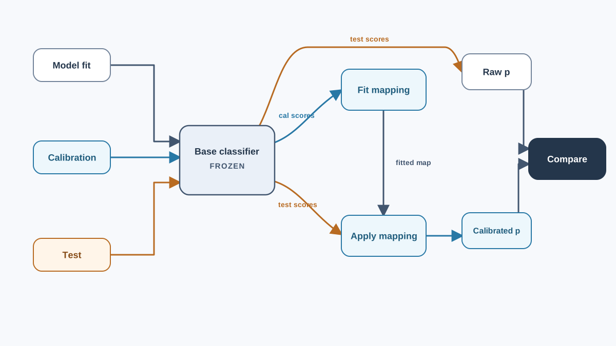
Here is where the design pays off. We split the training data once more, fit the base model on the model-training portion, and fit the calibrator on the calibration portion. The base model is not refit.
from sklearn.calibration import CalibratedClassifierCV
from sklearn.frozen import FrozenEstimator  # scikit-learn >= 1.6

X_fit, X_cal, y_fit, y_cal = train_test_split(
    X_train, y_train, test_size=0.4, stratify=y_train, random_state=42
)

base = RandomForestClassifier(n_estimators=300, random_state=42)
base.fit(X_fit, y_fit)

platt = CalibratedClassifierCV(
    FrozenEstimator(base), method="sigmoid", cv="prefit"
)
platt.fit(X_cal, y_cal)

isotonic = CalibratedClassifierCV(
    FrozenEstimator(base), method="isotonic", cv="prefit"
)
isotonic.fit(X_cal, y_cal)
On older scikit-learn versions, pass the fitted estimator directly with cv="prefit" instead of wrapping it in FrozenEstimator. Either way, the calibrator sees only X_cal — rows the base model never trained on.
The two methods differ in how flexible a mapping they allow:
- Platt scaling (
method="sigmoid") fits a sigmoid — a smooth, low-variance curve. It needs less calibration data and rarely overfits. - Isotonic regression (
method="isotonic") fits a monotonic step function. It is more flexible and can capture sharper corrections, but it overfits when calibration data is scarce.
The tradeoff is flexibility versus variance. With plenty of calibration rows, isotonic often wins. With few, Platt is the safer bet.
Common mistake: Using
CalibratedClassifierCV(base, cv=5)and calling the result a controlled comparison. That version refits the base model on each fold and averages five classifier-calibrator pairs, so the calibrated predictions come from a different training procedure than the raw ones. Any change in the diagram or Brier score is now a mix of calibration and a different ensemble. If you want to isolate calibration, freeze the base model and calibrate on held-out scores.
Knowledge check
Check your understanding
Answer this question before you continue.
Compare Reliability Diagrams and Brier Scores Side by Side
Now turn the two runs into evidence. Plot all three curves on the same axes:
raw_mp, raw_fp = reliability(y_test, raw_proba)
pl_mp, pl_fp = reliability(y_test, platt.predict_proba(X_test)[:, 1])
iso_mp, iso_fp = reliability(y_test, isotonic.predict_proba(X_test)[:, 1])

plt.plot([0, 1], [0, 1], "k--", label="perfect")
plt.plot(raw_mp, raw_fp, "o-", label="raw")
plt.plot(pl_mp, pl_fp, "s-", label="Platt")
plt.plot(iso_mp, iso_fp, "^-", label="isotonic")
plt.xlabel("mean predicted probability")
plt.ylabel("fraction of positives")
plt.legend()
plt.show()
Then report the Brier score for each on the same test set. The Brier score is a proper scoring rule: it rewards both calibration and sharpness, so it will not be gamed by a model that hedges every prediction toward 0.5.
for name, proba in [
    ("raw", raw_proba),
    ("Platt", platt.predict_proba(X_test)[:, 1]),
    ("isotonic", isotonic.predict_proba(X_test)[:, 1]),
]:
    print(name, round(brier_score_loss(y_test, proba), 4))
Interpret the result honestly. A lower Brier score is evidence of better probability quality, but a small gap on a small test set may not be meaningful. Check that ranking is preserved too. Because the calibrator is a monotonic map of the same fixed scores, AUC should stay essentially flat — a tiny shift is expected under isotonic ties, but a large swing means something else changed.
| Method | Flexibility | Data appetite | Typical failure mode |
|---|---|---|---|
| Raw | none | n/a | over-confident at the extremes |
| Platt (sigmoid) | low | modest | underfits a sharp correction |
| Isotonic | high | large | overfits sparse calibration data |
Failure Modes and Debugging Signals
Most broken calibration experiments fail quietly. Watch for these:
- Leakage. Calibrating on training rows, or tuning anything on the test set, inflates the apparent improvement. The calibrator must see held-out predictions only.
- Refit confusion. If you use
cv=5instead of a frozen base model, you are comparing two workflows, not isolating calibration. Decide which question you are asking before you read the numbers. - Empty or sparse bins. A reliability diagram with a few crowded bins and many empty ones is not evidence of anything. Raise the sample count or lower
n_bins. - Isotonic overfitting. A jagged, step-heavy curve that hugs the calibration split but does not generalize is the classic symptom. Compare against Platt before trusting it.
- Resampling side effects. Oversampling or undersampling the training set can distort calibration in ways the calibrator may not repair. If you resample, re-check the reliability diagram afterward.
- Class imbalance. With a rare positive class, bin counts get thin fast and the curve turns noisy. Read it with that in mind, and prefer more bins only when you have the samples to fill them.
Common mistake: Treating a lower Brier score as proof the model is "better." It is proof the probabilities are more reliable. If your downstream decision only needs a hard label at a fixed threshold, that improvement may not change a single outcome.
One Modification Worth Running
Copy-paste teaches recognition. One deliberate change teaches the mechanism. Pick one of these, state your prediction first, then run it:
- Change
n_binsfrom 10 to 5, then to 20. Watch how much of the curve shape is a binning artifact rather than a real miscalibration. - Swap the base estimator for a logistic regression and predict which direction the raw curve moves. A linear model is often closer to calibrated out of the box.
- Cut the calibration split size and watch isotonic degrade faster than Platt. This is the flexibility-versus-variance tradeoff made visible.
The gap between what you predicted and what you saw is the actual lesson. That gap is where your mental model gets corrected.
When Calibration Is Worth the Extra Step
Add calibration when the number itself drives a decision: expected cost calculations, risk scoring, ranking by predicted likelihood, or blending your probabilities with other estimates. In those cases an over-confident 0.9 quietly corrupts everything downstream.
Skip it when the only output is a hard class label at a fixed threshold, or when the model is already well calibrated. And remember the boundary: calibration does not fix a bad model. It reshapes scores; it does not add information the base model never captured.
Calibration is also a property of a model-plus-data combination, not a permanent upgrade. When the data distribution moves, the mapping you learned can drift out of date. Re-check it the same way you would re-check any other assumption.
The reusable rule: calibrate when the number drives a decision, verify it on data the calibrator never saw, and re-verify when the world shifts. The natural next experiment is to run this same comparison across several base estimators and see which ones arrive already trustworthy — because calibration is a diagnostic habit, not a one-time fix.
Knowledge check
Final check
Finish the article by checking the ideas you just learned.
References
Build stronger machine learning foundations
Use structured resources to connect theory, scikit-learn workflows, and evaluation practice.


