How DBSCAN Forms Clusters: Density Reachability and Connectivity

Two points sit the same distance from a dense blob. DBSCAN labels one a cluster member and the other noise. That looks arbitrary until you stop asking how close a point is to the cluster and start asking who is allowed to reach whom.

If you already know what DBSCAN is for — dense groups, a noise label, the eps and min_samples knobs — this article fills in the machinery underneath. By the end, you should be able to take any point in a small dataset and trace its label by hand using three definitions. No library required.

Notation: Points, Radius, and the Neighborhood Set

Before any rule makes sense, fix the symbols.

Let $D$ be your dataset: $n$ points in $\mathbb{R}^d$. Let $\text{dist}(x, y)$ be a distance function, usually Euclidean. The $\varepsilon$-neighborhood of a point $x$ is the set of dataset points within radius $\varepsilon$:

$N_\varepsilon(x) = \{\, y \in D : \text{dist}(x, y) \le \varepsilon \,\}$

Three details in that line matter more than they look.

The boundary is inclusive. A point exactly $\varepsilon$ away is inside the neighborhood. The point $x$ itself is normally counted, so $x \in N_\varepsilon(x)$.

The neighborhood is defined over the dataset, not over continuous space. DBSCAN only ever sees the points you gave it. A region that is empty in reality but dense in your sample will be treated as dense, because the algorithm has no other evidence.

The second parameter, min_samples (called MinPts in the original formulation), is the density threshold. Higher min_samples or lower eps means a point must be more crowded to count as dense.

Warning: eps is measured in the units of your features. If one column ranges over thousands and another over single digits, the neighborhood set is dominated by the large-scale feature. Scale your features before you interpret any of the definitions below.

The Core-Point Condition

Everything else in DBSCAN hangs on one predicate, and that predicate is local. It says nothing about clusters. It only asks how crowded the space immediately around a single point is.

A point $x$ is a core point if:

$|N_\varepsilon(x)| \ge \text{min\_samples}$

A border point is not core, but lies inside the neighborhood of at least one core point. A noise point is neither.

That is the whole classification. Core, border, noise — decided one point at a time.

A worked count

Take four points on a line: $A$ at 0, $B$ at 1, $C$ at 2, and $D$ at 6. Set $\varepsilon = 1.5$ and min_samples = 3.

• $N_\varepsilon(A) = \{A, B\}$ — size 2. Not core.
• $N_\varepsilon(B) = \{A, B, C\}$ — size 3. Core.
• $N_\varepsilon(C) = \{B, C\}$ — size 2. Not core.
• $N_\varepsilon(D) = \{D\}$ — size 1. Not core.

$B$ is the only core point. $A$ and $C$ are within $\varepsilon$ of $B$, so they are border points. $D$ is far from everything, so it is noise.

Common mistake: counting neighbors while excluding the point itself. Many implementations include the point in its own neighborhood count, so excluding it silently shifts your effective threshold by one. If your hand count disagrees with the library, check this first.

Notice what just happened. $A$ and $C$ are members of a cluster not because they are dense, but because a dense point is nearby. The core condition is what makes DBSCAN density-based rather than distance-based: a point qualifies by how crowded its surroundings are, not by where it sits.

Direct Density-Reachability and Why It Is Asymmetric

Now connect points. The one-step relation is called direct density-reachability.

A point $y$ is directly density-reachable from $x$ if both hold:

1. $y \in N_\varepsilon(x)$ — proximity.
2. $x$ is a core point — density.

Read those as a gate with two locks. Proximity alone is not enough: a border point cannot reach its neighbors just because they are close. Density alone is not enough either: a core point cannot reach points outside its radius.

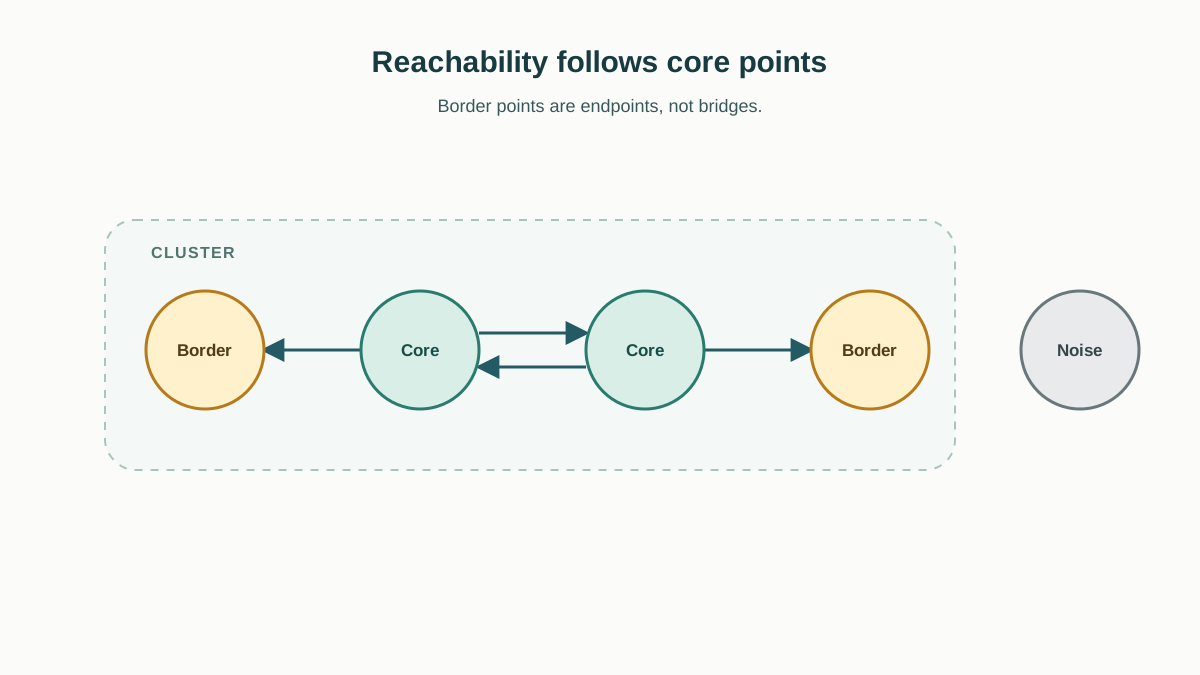
The asymmetry falls straight out of clause 2. The relation requires the source to be core. So a border point can be reached, but it can reach nothing. In the example above, $A$ is directly density-reachable from $B$, but $B$ is not directly density-reachable from $A$, because $A$ is not core.

Direction matters because the density anchor sits on one side only. Reachability is a one-way street, and the arrow always points away from density.

There is a clean boundary worth stating precisely. With a symmetric distance function and a shared $\varepsilon$, the neighborhood relation itself is symmetric: if $y \in N_\varepsilon(x)$, then $x \in N_\varepsilon(y)$. So two core points within $\varepsilon$ of each other are mutually directly reachable. The asymmetry appears only when the source is not core — a core point can reach a nearby border point, but the border point cannot reach back.

Picture it as a diagram: draw a dashed circle of radius $\varepsilon$ around each point. Draw an arrow from every core point to each point inside its circle. No arrows leave border points. The picture is the definition.

Density-Reachability as a Chain

One step is not enough to describe a cluster that spans a region. So extend the relation into a path.

A point $y$ is density-reachable from $x$ if there is a chain

$x = p_1, \; p_2, \; \dots, \; p_n = y$

where each $p_{i+1}$ is directly density-reachable from $p_i$.

Every link in that chain — except possibly the last — must be a core point. That is the constraint that keeps the path inside dense territory. You can step from core to core to core, and then take one final step onto a border point. You cannot step through a border point to reach anything beyond it.

Tracing the chain

Return to the line example and add a point $E$ at 3.5, with $\varepsilon = 1.5$ and min_samples = 3. Recompute every neighborhood that changes.

• $N_\varepsilon(C) = \{B, C, E\}$ — size 3. $C$ is now core.
• $N_\varepsilon(E) = \{C, E\}$ — size 2. Not core.

So the chain extends: $B$ reaches $C$ directly, and $C$ — now core — reaches $E$ directly. $E$ is a border point of the cluster. The chain from $B$ reaches $C$, then $E$, and stops there, because no core point exists to bridge the gap toward $D$.

That stopping point is the cluster boundary. The cluster is exactly the set of points reachable from a core point, and the boundary is exactly where density fails. No core point, no bridge, no crossing.

This is the trap in hand-tracing DBSCAN. Adding one point can promote an existing point from border to core, which changes the reachability graph everywhere downstream. Recompute the neighborhoods of every point near the change, not just the new point.

Reachability is still not symmetric after chaining. The asymmetry from the one-step relation survives transitivity: if $y$ is reachable from $x$ through a chain, $x$ is generally not reachable from $y$, because the chain's direction is fixed and the last point may not be core.

Density-Connectivity: Making Membership Symmetric

Reachability alone cannot define a cluster, because it is one-way. Two border points on opposite sides of a dense core are both reachable from that core, but neither is reachable from the other. If membership depended on reachability, they would land in different clusters — which is wrong.

So DBSCAN introduces a symmetric relation. Two points $x$ and $y$ are density-connected if there exists some point $o$ such that both $x$ and $y$ are density-reachable from $o$.

The shared anchor $o$ is the entire trick. It converts a one-way relation into a two-way one. If $x$ and $y$ share an anchor, the direction of each individual chain stops mattering.

Concretely: two border points on opposite sides of a dense core are not reachable from each other, yet they are density-connected through a common core point. So they land in the same cluster. That is how DBSCAN builds elongated, non-spherical clusters — the connection travels through the dense region, not across the gap.

Keep the two relations separate in your head or the cluster definition will not parse.

Relation	Symmetric?	Role
Neighborhood $N_\varepsilon(x)$	Yes	Defines "nearby"
Core condition	N/A (a predicate)	Identifies dense regions
Direct density-reachability	No	Single-step connections
Density-reachability	No	Multi-step paths
Density-connectivity	Yes	Cluster membership

The Cluster Definition: Maximality and Connectivity

Now assemble the pieces. A cluster $C$ is a non-empty subset of $D$ satisfying two properties:

Maximality. If $x \in C$ and $y$ is density-reachable from $x$, then $y \in C$.

Connectivity. Every pair of points in $C$ is density-connected.

Each property rules out a different failure. Maximality prevents splitting one dense region into two clusters: if you can reach a point from inside the cluster, that point belongs to the cluster. Connectivity prevents merging two dense regions across a gap: every pair in the cluster must be linked through a shared anchor, so a low-density gap severs the connection.

Noise is simply the complement: points that are not density-reachable from any core point.

This definition is descriptive, not constructive. It tells you what a valid cluster is. It does not tell you how to find one. The algorithm's breadth-first expansion from core points is one way to compute a set that satisfies the definition — but the definition came first.

Note: The formal definition does not fully pin down border-point assignment. A border point within $\varepsilon$ of core points from two different clusters can legitimately be assigned to either one, and the assignment can depend on the order in which the data is traversed. The core points are always assigned consistently; the border points are the loose end.

What the Definitions Predict in Practice

The formal structure is not decoration. It predicts exactly what you will see when you run the algorithm.

Chains of core points are the only bridges between dense regions. A single low-density gap splits a cluster, no matter how close the two sides look on a scatter plot. If you see two blobs that "should" be one cluster, count the core points between them. If there are none, DBSCAN is right and your eye is wrong.

Border points are the fragile edge of a cluster. They are members by courtesy of a nearby core point. Change eps, change min_samples, or reorder your rows, and a border point can flip labels or drop to noise. If a point's membership matters to your conclusion, check whether it is core or border before you trust it.

Cluster size is driven by core points, not total points. Because reachability is directional, a point can be a member without being able to pull any other point in. A cluster with a thousand border points and one core point is a cluster with one point of structural support.

When this model is the right tool: clusters of arbitrary shape, unknown cluster count, and a genuine noise category. When it is not: strongly varying densities in one dataset (a single global eps cannot serve both a tight cluster and a loose one), or any situation where you need every point assigned to something.

Here is the practical check I would give anyone learning this: before trusting a label, ask which core point reached this point, and by what chain. If you cannot answer, the label is a library output, not an explanation.

Where to Go Next

The decision rule is short. A point belongs to a cluster only if a core point can reach it. Two points share a cluster only if some core point reaches both.

That rule is easy to state and easy to forget the moment you are staring at a plot. So make it concrete: take a small dataset, run DBSCAN, and then vary eps and min_samples one at a time. At each setting, inspect the neighborhood count and core-sample status of the points you care about. A point can change type — core, border, or noise — when the parameters move, so a label flip does not by itself tell you what the point was before. What you are looking for is the mechanism: which points gained or lost enough neighbors to cross the core threshold, and which border points shifted assignment because they sit near core points from two clusters. The theory stops being abstract the moment you can point to the count that changed and explain why the label followed.