
How Class Prevalence Changes Precision and the PR Baseline
A model can keep the same weights, the same features, and the same threshold, and still report precision 0.9 on your test set and precision 0.3 in…

Key topics
A model can keep the same weights, the same features, and the same threshold, and still report precision 0.9 on your test set and precision 0.3 in production. Nothing about the classifier changed. What changed is how many positives were in the pool it was scored against.
That gap is not a bug, and it is not a sign that your test set was "wrong." It is arithmetic. Precision is not a property of the classifier alone. It is a property of the classifier's output measured against a specific class mix. Once you see the algebra, the production surprise stops being mysterious and starts being predictable.
This article derives that algebra from first principles. We will express precision as a function of prevalence, recall, and false-positive behavior, work a numerical example you can check by hand, and then derive the no-skill baseline for a precision-recall curve. Along the way we will draw a hard line between three things people constantly confuse: prevalence effects, threshold choice, and classifier quality.
If you need a refresher on what precision, recall, and a PR curve are, the comparison of ROC and precision-recall curves covers that ground. Here we go straight to the mechanism.
Why the Same Model Reports Different Precision
Picture two evaluation runs. Same trained model. Same decision threshold. Same code path.
In run A, the scored population is balanced: half positives, half negatives. Precision comes back at 0.9.
In run B, the scored population is skewed: 1% positives, 99% negatives. Precision comes back at 0.3.
The default belief is that precision measures the classifier. Under that belief, the two runs should agree, and any disagreement means something is broken. The correction is sharper: precision measures the classifier's output against a specific class mix. Change the mix, and you change the number, even when the model's behavior is identical.
Three quantities do all the work in this article:
- Prevalence (π): the share of actual positives in the population you score.
- Recall: the share of actual positives the model catches.
- False-positive behavior: how often the model fires on actual negatives.
Everything else follows. One scope note before we start: this is a derivation about binary classification with a fixed decision rule. Prevalence is not the only thing that matters in evaluation. It is the thing that makes precision move when nothing else did.
Notation and the Confusion Matrix We Will Use
Before the equations, pin down the symbols. Every one of them maps to something you can count in a confusion matrix.
| Symbol | Meaning |
|---|---|
| TP | Actual positives predicted positive |
| FP | Actual negatives predicted positive |
| FN | Actual positives predicted negative |
| TN | Actual negatives predicted negative |
| P | Total actual positives, P = TP + FN |
| N | Total actual negatives, N = FP + TN |
From those counts, two rates matter here:
- Recall, also called the true positive rate: TPR = TP / (TP + FN) = TP / P.
- False-positive rate: FPR = FP / (FP + TN) = FP / N.
And one property of the population:
- Prevalence: π = P / (P + N), the fraction of the scored population that is actually positive.
Three assumptions hold the derivation together. First, labels are binary. Second, the threshold is fixed, so the model sits at one operating point with one recall and one FPR. Third, the class mix of the scored population is known or assumed.
That third assumption is the one that breaks in practice. π is a property of the data you score on, not of the model. Your training set, your test set, and your production stream can each have a different π, and precision will follow each one.
Knowledge check
Check your understanding
Answer this question before you continue.
Deriving Precision From Prevalence, Recall, and FPR
Start from the definition:
The numerator is the mass of true positives. The denominator is everything the model called positive. Now rewrite both in terms of rates instead of raw counts.
The true positives are the positives the model caught. There are P actual positives, and it catches a fraction equal to recall:
The false positives are the negatives the model fired on. There are N actual negatives, and it fires on a fraction equal to FPR:
Substitute both into the precision definition:
Now divide numerator and denominator by the total population size, P + N. This is the step that turns raw counts into shares. The positive count becomes prevalence, and the negative count becomes its complement:
That is the precision recall prevalence formula in its working form. Read it in words and the structure is almost physical. The numerator is the true-positive mass. The denominator adds the false-positive mass. Prevalence, π, sets how much weight each side carries.
Two consequences fall straight out of the algebra:
- As π shrinks, the numerator shrinks with it, but the FPR term is scaled by (1 − π), which grows toward 1. The false-positive mass holds its ground while the true-positive mass evaporates.
- Recall is prevalence-free by construction. It is TP / P, and P cancels out of the ratio. That is exactly why precision is the metric that moves when the class mix changes, and recall is not.
Knowledge check
Check your understanding
Answer this question before you continue.
A Worked Example: Same Recall, Three Prevalences
Numbers make the direction and the size of the effect concrete. Hold the model fixed at recall = 0.8 and FPR = 0.1. These are the model's behavior, and they do not change across the three rows. Only π changes.
| Prevalence (π) | recall × π | FPR × (1 − π) | Precision |
|---|---|---|---|
| 0.50 | 0.400 | 0.050 | 0.889 |
| 0.10 | 0.080 | 0.090 | 0.471 |
| 0.01 | 0.008 | 0.099 | 0.075 |
Check the middle row by hand. recall × π = 0.8 × 0.1 = 0.08. FPR × (1 − π) = 0.1 × 0.9 = 0.09. Precision = 0.08 / (0.08 + 0.09) = 0.08 / 0.17 ≈ 0.471. The other rows follow the same two multiplications and one division.
The model never changed. Recall stayed at 0.8. FPR stayed at 0.1. Yet precision fell from 0.889 to 0.075 — a collapse of more than an order of magnitude — purely because positives became rare.
The mechanism is worth saying plainly. At low prevalence, the negative pool is enormous. A 10% false-positive rate applied to a huge pool of negatives generates a large absolute number of false positives. Those false positives pile into the denominator and swamp the handful of true positives the model managed to catch. The model is not worse. The room it is standing in got bigger, and the noise scaled with the room.
Knowledge check
Check your understanding
Answer this question before you continue.
The No-Skill Baseline Is Not 0.5
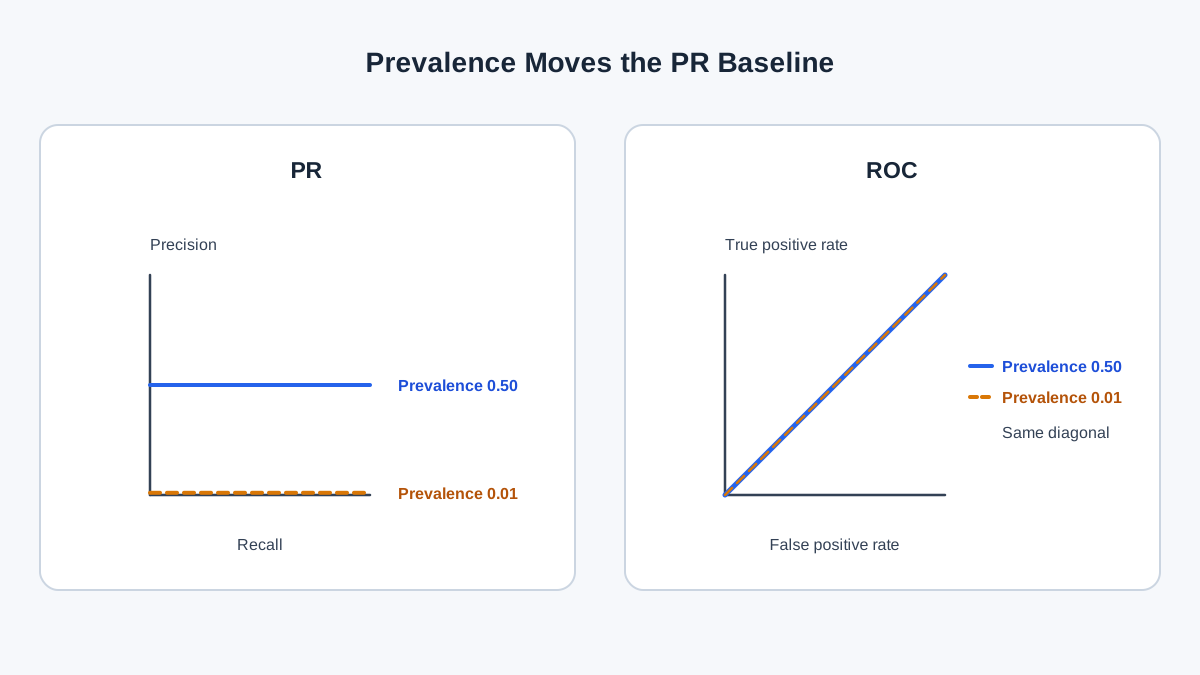
Now the part that trips up almost everyone reading a PR curve.
Define a no-skill classifier as one that assigns positive labels independently of the true label — random guessing at a fixed rate. It has no information about which cases are actually positive.
What precision does such a classifier achieve? If the label it assigns is independent of the truth, then among the cases it calls positive, the proportion that are actually positive is just the base rate of positives in the population. That is π. This holds at every recall level, because the classifier's guesses carry no signal regardless of how many it makes.
So the no-skill PR curve is a horizontal line at precision = π, not at 0.5.
Contrast this with ROC. On an ROC plot, the no-skill classifier traces the diagonal from (0,0) to (1,1) — a fixed reference that does not depend on the class mix. That structural difference is the reason the two plots diverge under imbalance. ROC's baseline is anchored to the geometry of the rates. PR's baseline is anchored to the prevalence of your data.
The practical consequence is blunt. An AUPRC of 0.4 on a 1% prevalence problem sits far above its 0.01 baseline. The same 0.4 on a balanced problem sits near chance, because the baseline there is 0.5. The number is identical; the meaning is opposite. Always read a PR curve against its own baseline, never against a memorized threshold like 0.5.
Knowledge check
Check your understanding
Answer this question before you continue.
What This Algebra Does Not Explain
The derivation is powerful, and it is also narrow. Knowing where it stops is part of using it well.
Prevalence changes the scale of precision. It does not tell you whether the model ranks well. A model can have high precision at low prevalence purely because the baseline is low. Before celebrating, check the lift over π. A model can also have low precision at high prevalence while still being a strong ranker — precision alone is not a quality verdict.
Threshold choice and prevalence are two different levers. Moving the threshold slides you along a single PR curve, trading precision against recall at a fixed π. Changing prevalence, by contrast, changes the precision you observe at a fixed operating point — the formula above tells you exactly how much. The curve-level picture is subtler: if you hold the model's class-conditional score distributions fixed and only change the class mix of the scored population, the entire PR curve shifts and its baseline moves with it. But that clean shift is an assumption, not a guarantee. Resampling, reweighting, or a genuine population shift can also change how the model's scores behave conditional on class, in which case the curve is not simply translated — it is reshaped. People conflate these constantly: they see precision drop, reach for the threshold, and miss that the population underneath them changed. One lever is inside the model's control at scoring time. The other is a fact about the world you are scoring.
If you want the broader picture of how to choose among metrics and plots for a given cost structure, that belongs to the wider evaluation curriculum. Here we stay on the algebra, because the algebra is what tells you which lever you are actually pulling.
Using the Formula in Practice
Turn the derivation into a decision rule you can apply to your own evaluation setup.
Before you trust any precision number, ask what prevalence it was computed at — and whether that matches the population you will deploy on. If your test set is balanced but production is not, your test precision is a number about a world you do not live in.
If you resample or reweight your test set, you have changed π, and therefore changed precision. That is fine as long as you report the prevalence alongside the metric. A precision of 0.47 means nothing until you say it was measured at π = 0.1.
You can verify the formula against your own scores with a short check. Take one set of predicted scores, fix a threshold, and compute precision twice: once on the natural class mix, once on a resampled mix. The formula predicts the shift before you run it.
import numpy as np
from sklearn.metrics import precision_score

rng = np.random.default_rng(0)
n = 100_000
# Simulate scores: positives score higher on average, but overlap exists.
y = (rng.random(n) < 0.01).astype(int)          # 1% prevalence
scores = rng.normal(loc=0.3 * y, scale=1.0, size=n)
threshold = 0.5
y_pred = (scores > threshold).astype(int)

# Natural mix
p_natural = precision_score(y, y_pred, zero_division=0)

# Reweight to a balanced mix by resampling positives and negatives equally
pos_idx = np.flatnonzero(y == 1)
neg_idx = np.flatnonzero(y == 0)
k = min(len(pos_idx), len(neg_idx))
balanced = np.concatenate([
    rng.choice(pos_idx, k, replace=False),
    rng.choice(neg_idx, k, replace=False),
])
p_balanced = precision_score(y[balanced], y_pred[balanced], zero_division=0)

print(f"prevalence ~0.01 -> precision {p_natural:.3f}")
print(f"prevalence ~0.50 -> precision {p_balanced:.3f}")
The two printed numbers will differ, and the formula tells you why before you look. The model's recall and FPR are roughly constant across the two runs; only π moved.
The rule of thumb that follows: report precision, recall, and prevalence together, or report precision as lift over the π baseline. A bare precision number is an incomplete measurement, because it silently depends on a quantity you did not state.
Where to Go Next
Collapse everything above into one sentence you can carry: precision is a joint property of the model and the population, so any precision number without its prevalence is a measurement with a missing variable.
Your next practical step is to recompute your own evaluation at the prevalence you actually expect in deployment, then compare the result against the π baseline rather than against 0.5. Treat that comparison as context, not as a verdict. A thin lift over baseline at one operating point does not prove the model has no useful ranking behavior — it tells you to inspect the full PR curve and the region of the curve you actually plan to operate in. A large lift at one point does not prove the model is strong everywhere either. Read the curve, not a single number, and you will know which lever you are pulling.
Knowledge check
Final check
Finish the article by checking the ideas you just learned.
References
Build stronger machine learning foundations
Use structured resources to connect theory, scikit-learn workflows, and evaluation practice.


