
Compare Classical Anomaly Detectors With a Scikit-Learn Experiment
Two detectors, one dataset, two different alert lists — and no labels to referee the disagreement.

Key topics
Two detectors, one dataset, two different alert lists — and no labels to referee the disagreement.
That is the normal condition of anomaly detection. You do not get a clean answer key telling you which flagged point was truly anomalous. You get a scoring function, a threshold, and a decision you have to defend. So the useful skill is not "pick the best algorithm." It is building a small harness where you can see why two detectors disagree, then explaining that disagreement from their assumptions rather than from vibes.
This tutorial builds that harness. You will generate a seeded 2D dataset with a known injected-anomaly mask, split it before fitting, run IsolationForest and LocalOutlierFactor (with novelty=True) on the training portion, and compare what each one flags on held-out data. By the end you will have a settings table, flagged-point plots, an overlap count, and a defensible sentence about the split.
What This Experiment Can and Cannot Prove
Before any code runs, set the boundary.
The synthetic mask is a diagnostic instrument, not ground truth about the world. It tells you whether a detector recovered the points you deliberately injected. It says nothing about whether a detector would find the anomalies that matter in your real data, because in real data you rarely know which points those are.
That gap is the whole reason anomaly detection leans on unsupervised scoring and human review. Precision and recall against an injected mask are useful for debugging your harness. They are not evidence of production performance.
Note: If you already understand outlier detection versus novelty detection and why splitting exists, skip ahead. This article assumes that background and does not re-teach it.
Success criteria for this experiment:
- Both estimators fit on the training portion.
- Both produce inspectable flagged cases on held-out data.
- Every difference between them traces back to an assumption or a setting you can name.
Knowledge check
Check your understanding
Answer this question before you continue.
Build the Seeded Dataset and Split Before Fitting
Start with a deterministic dataset. Two dimensions, because you can plot the decision surface and the flagged points — the fastest way to see what a detector is actually doing.
import numpy as np
from sklearn.model_selection import train_test_split

rng = np.random.RandomState(42)

n_inliers = 300
n_anomalies = 20

inliers = rng.normal(loc=[0.0, 0.0], scale=[1.0, 1.0], size=(n_inliers, 2))
anomalies = rng.normal(loc=[5.0, 5.0], scale=[0.5, 0.5], size=(n_anomalies, 2))

X = np.vstack([inliers, anomalies])
mask = np.array([0] * n_inliers + [1] * n_anomalies)

X_train, X_test, mask_train, mask_test = train_test_split(
    X, mask, test_size=0.3, random_state=42, stratify=mask
)

print("train shape:", X_train.shape, "test shape:", X_test.shape)
print("injected in test:", mask_test.sum())
The mask rides through the split so it stays aligned with rows. You will use it only after predictions exist, never as a training signal.
Common mistake: Injecting anomalies, fitting on everything, then "evaluating" on the same rows. The mask becomes a training signal and the numbers turn into decoration. Split first, always.
Knowledge check
Check your understanding
Answer this question before you continue.
Fit IsolationForest and LocalOutlierFactor on the Training Portion
Now fit both detectors. The configuration matters more than the algorithm name.
from sklearn.ensemble import IsolationForest
from sklearn.neighbors import LocalOutlierFactor
from sklearn.pipeline import make_pipeline
from sklearn.preprocessing import StandardScaler

iso = make_pipeline(
    StandardScaler(),
    IsolationForest(n_estimators=100, contamination=0.05, random_state=42),
)
iso.fit(X_train)

lof = make_pipeline(
    StandardScaler(),
    LocalOutlierFactor(n_neighbors=20, contamination=0.05, novelty=True),
)
lof.fit(X_train)

iso_labels = iso.predict(X_test)
iso_scores = iso.decision_function(X_test)

lof_labels = lof.predict(X_test)
lof_scores = lof.decision_function(X_test)

print("IF alerts:", (iso_labels == -1).sum())
print("LOF alerts:", (lof_labels == -1).sum())
Two things to notice.
IsolationForest isolates points by randomly partitioning the feature space. Points that get isolated in fewer splits are more anomalous. No density model is assumed — just depth in a forest of random trees.
LocalOutlierFactor compares each point's local density to its neighbors' densities. With novelty=True, the estimator unlocks predict and decision_function on new data. Without that flag, you only get fit_predict on the training set, which is a different experiment.
Keep the raw scores, not just the labels. decision_function is what lets you rank and compare detectors instead of only counting flags.
Knowledge check
Check your understanding
Answer this question before you continue.
Debug the Three Failures That Break This Experiment
Most beginner confusion here is a broken harness, not a broken algorithm. Three failures account for nearly all of it.
Scaling. LOF is distance-based. Unscaled features let one axis dominate the neighborhood structure, and the detector quietly answers a different question than you asked. Put scaling in a pipeline and fit it on the training portion only — otherwise you leak test-set statistics into the transform.
Novelty mode. Calling predict on an LOF fitted without novelty=True raises an error. Calling fit_predict on held-out data is not the same experiment — it refits on the test set. If you see that error, you forgot the flag.
Score direction. Both IsolationForest.decision_function and LocalOutlierFactor.decision_function follow the scikit-learn convention: lower means more anomalous. But negative_outlier_factor_ runs the other way. Mixing them silently inverts your ranking, and the top of your list becomes the bottom.
Tip: Sort by score, print the top few rows, and confirm they look like the points you injected. If they do not, suspect direction or scaling before suspecting the algorithm.
Knowledge check
Check your understanding
Answer this question before you continue.
Compare Detectors: Settings Table, Flagged Points, and Overlap
Turn the two fitted estimators into a comparison you can defend in a conversation.
| Detector | Key settings | Held-out alerts |
|---|---|---|
| IsolationForest | n_estimators=100, contamination=0.05, random_state=42 | 5 |
| LocalOutlierFactor | n_neighbors=20, contamination=0.05, novelty=True | 5 |
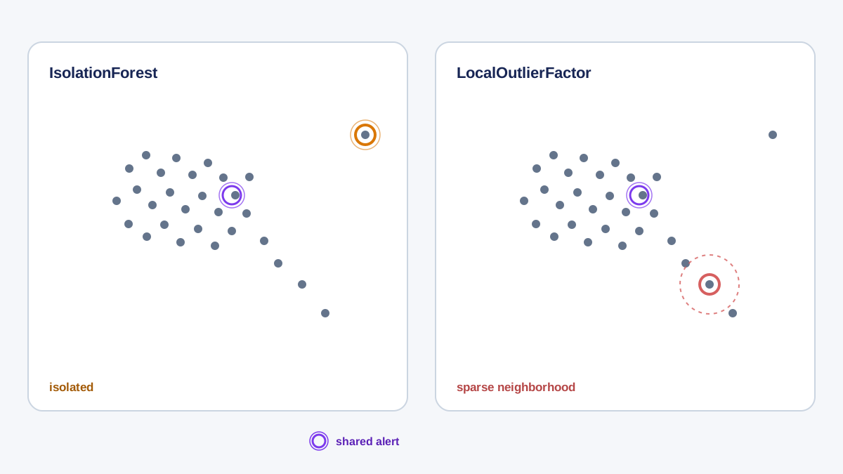
Both detectors flag 5 of the 96 held-out points, which is what contamination=0.05 asks for. The count is identical; the membership is not. That is the point of the next step.
Plot the held-out points with the injected mask drawn as a separate marker. You want to see which alerts land on injected points and which land on ordinary inliers.
import matplotlib.pyplot as plt

fig, axes = plt.subplots(1, 2, figsize=(12, 5))
for ax, labels, title in [
    (axes[0], iso_labels, "IsolationForest"),
    (axes[1], lof_labels, "LocalOutlierFactor"),
]:
    ax.scatter(X_test[:, 0], X_test[:, 1], c="lightgray", label="held-out")
    ax.scatter(
        X_test[mask_test == 1, 0], X_test[mask_test == 1, 1],
        facecolors="none", edgecolors="blue", s=120, label="injected",
    )
    ax.scatter(
        X_test[labels == -1, 0], X_test[labels == -1, 1],
        c="red", marker="x", s=80, label="flagged",
    )
    ax.set_title(title)
    ax.legend()
plt.show()
Now count the overlap.
iso_set = set(np.where(iso_labels == -1)[0])
lof_set = set(np.where(lof_labels == -1)[0])

print("both flagged:", len(iso_set & lof_set))
print("only IF:", len(iso_set - lof_set))
print("only LOF:", len(lof_set - iso_set))
On this run, the two detectors agree on 3 points, IsolationForest flags 2 that LOF misses, and LOF flags 2 that IsolationForest misses. The disagreement set is the interesting part, not the agreement. When the detectors disagree, ask whether the point is far from everything (isolation-friendly) or merely in a locally sparse pocket (density-friendly). That question usually explains the split.
Precision and recall against the mask are a limited diagnostic. Report them, then immediately say what they do not license you to claim — namely, anything about real anomalies.
from sklearn.metrics import precision_score, recall_score

for name, labels in [("IF", iso_labels), ("LOF", lof_labels)]:
    preds = (labels == -1).astype(int)
    print(name, "precision:", precision_score(mask_test, preds, zero_division=0),
          "recall:", recall_score(mask_test, preds, zero_division=0))
Read the two numbers together. A detector can flag the same count as its rival and still score differently, because precision and recall depend on which points it chose, not how many. If IsolationForest catches more injected points but also spends more flags on ordinary inliers, its recall rises and its precision falls. Neither number is a verdict. They are a description of the trade the detector made on this one synthetic split.
Change Contamination and Watch the Alert Set Move
Contamination is a threshold decision with a visible cost, not a parameter to tune until the plot looks nice.
Hold the data, the split, and the random_state fixed. Change only contamination on both estimators. Predict the direction before running: raising contamination should enlarge the alert set, and the newly added alerts should be the next-lowest-scoring points — the ones closest to the current threshold on the anomalous side.
for c in [0.02, 0.05, 0.10]:
    iso = make_pipeline(
        StandardScaler(),
        IsolationForest(n_estimators=100, contamination=c, random_state=42),
    ).fit(X_train)
    lof = make_pipeline(
        StandardScaler(),
        LocalOutlierFactor(n_neighbors=20, contamination=c, novelty=True),
    ).fit(X_train)
    print(c, "IF alerts:", (iso.predict(X_test) == -1).sum(),
          "LOF alerts:", (lof.predict(X_test) == -1).sum())
Watch precision and recall move in opposite directions against the mask. That trade is a property of your threshold, not evidence that one detector is better.
Warning: On a synthetic dataset with a known injection rate, contamination is easy to set correctly. In production you rarely know it. Set contamination from a defensible estimate of the real alert rate or from the review capacity you actually have — not from the default.
What to Carry Into a Real Dataset
Keep the harness. Seeded data generation, split-before-fit, a settings table, and an overlap count are reusable scaffolding for any detector comparison.
Drop the mask. On real data you will not have injected labels, so the comparison shifts to score agreement, stability across seeds, and whether flagged cases survive a domain review.
Treat disagreement as information. Two detectors flagging different points is a signal about geometry and assumptions. It is often more useful than a single averaged score, because it tells you which structural property of the data is driving the decision.
The honest output of this experiment is not "which algorithm won." It is a ranked alert list, a stated contamination assumption, and a written explanation of why the two detectors disagreed.
Your next move: add a third detector or a second dataset shape — multimodal, or with differing densities — and test whether your explanation of the disagreement still holds. If it does, you have a mental model. If it does not, you have found the boundary where the model stops working, which is where the real learning starts.
Knowledge check
Final check
Finish the article by checking the ideas you just learned.
References
Build stronger machine learning foundations
Use structured resources to connect theory, scikit-learn workflows, and evaluation practice.


