
Derive Local Outlier Factor From Local Reachability Density
A point can sit closer to its neighbors than anything else in the dataset and still be the anomaly. That is the contradiction Local Outlier Factor was…

Key topics
A point can sit closer to its neighbors than anything else in the dataset and still be the anomaly. That is the contradiction Local Outlier Factor was built to resolve.
Most of us start with the same mental model: an outlier is a point far from everything. Compute the distance to the mean, or to the nearest neighbor, sort, and flag the tail. That model works fine when your data has one density. It falls apart the moment your dataset contains a tight cluster and a loose scatter at the same time.
This article derives LOF from the ground up. We will define the notation, build reachability distance, turn it into local reachability density, and finish with the density ratio that produces the score. Then we will compute a small example by hand so the formulas stop being symbols and become arithmetic you can check.
If you have not yet framed outlier detection versus novelty detection, treat that as assumed background here. The short version: LOF is an unsupervised outlier-detection method. It scores the data it was trained on. By default it has no predict for new points.
Why Distance Alone Fails
Picture two clusters. On the left, points packed tightly together. On the right, points spread out with visible gaps. Now place two candidates: one just outside the tight cluster, one sitting comfortably inside the sparse cluster.
The point near the tight cluster is close to its neighbors in absolute terms. The point in the sparse cluster is far from its neighbors in absolute terms. A global distance rule flags the sparse point. But the sparse point belongs there — it is exactly as isolated as everything around it. The point hovering just outside the tight cluster does not belong. Its neighbors are packed; it is not.
That is the failure mode. Global distance methods assume one density. Real data has many.
LOF replaces the absolute question with a relative one. Instead of asking "how far is this point from everything?", it asks "how does this point's local density compare to the density of its neighbors?" A point is anomalous when it is sparser than the region it lives in — not when it is far from the origin.
This is what makes LOF a density-based anomaly detection method rather than a distance-threshold method. The score is a ratio, and ratios cancel out the scale of the region.
Knowledge check
Check your understanding
Answer this question before you continue.
Notation and the k-Nearest Neighborhood
Before any formula, fix the symbols. Every later equation maps back to one of these objects.
- k — the number of neighbors. You choose it. It is the single most important knob in the algorithm.
- p — the point we are scoring.
- N_k(p) — the set of k-nearest neighbors of p.
- k-distance(p) — the distance from p to its k-th nearest neighbor. This is the radius of p's neighborhood.
- d(p, o) — the distance between points p and o under whatever metric you picked.
One subtlety that trips people up: N_k(p) can contain more than k points. If several points sit at exactly the k-th distance, all of them are included. The set is defined by the distance, not by a count. This matters for tie handling, and it is one of the places where a hand calculation and a library call will quietly disagree.
The other assumption hiding in the notation is that distances are meaningful. If your features are on wildly different scales, the largest-range feature dominates the metric and the rest are noise. Scale first. And if you have mixed or categorical features, you need a metric you can defend — Euclidean distance on one-hot encoded categories is a choice, not a default.
Common mistake: Skipping feature scaling and then blaming LOF for a bad ranking. The algorithm measures distances. If the distances are wrong, the scores are wrong.
Reachability Distance: Smoothing the Neighborhood
Here is the first real formula:
reach-dist_k(p, o) = max( k-distance(o), d(p, o) )
Read it as a floor. If o is already inside its own k-neighborhood, then any point p near o is treated as being at least k-distance(o) away — even if p is closer than that.
Why bother? Because without the floor, tiny distance differences between points packed tightly around o would blow up the density estimate. The floor smooths those fluctuations. The larger k is, the more smoothing you get.
Now the part that catches almost everyone: the function is not symmetric. reach-dist_k(p, o) is generally not equal to reach-dist_k(o, p). The k-distance term belongs to the second argument. When you compute the reachability distance from p to o, you use o's k-distance, not p's.
Common mistake: Using
k-distance(p)instead ofk-distance(o). That variant is a different method — sometimes called Simplified-LOF — and it produces different scores. If your hand calculation disagrees with a library, check this first.
This is the same core-distance idea that shows up in DBSCAN, where a point's neighborhood radius defines how it reaches its neighbors. LOF borrows the concept and uses it to stabilize density estimates rather than to grow clusters.
Knowledge check
Check your understanding
Answer this question before you continue.
Local Reachability Density
With reachability distance in hand, define local reachability density:
lrd_k(p) = |N_k(p)| / Σ_{o ∈ N_k(p)} reach-dist_k(p, o)
In plain language: it is the inverse of the average reachability distance from p to its neighbors. High lrd means p sits in a dense region. Low lrd means p sits in a sparse one.
The direction is the part worth pausing on. This is the distance at which p can be reached from its neighbors — not the average distance from p outward. That sounds like a technicality until you remember the asymmetry. Because the reachability distance uses the neighbor's k-distance, the sum is measuring how tightly the neighborhood closes in around p.
Two consequences follow directly:
- Higher lrd → denser local region.
- Lower lrd → sparser local region.
There is one edge case you should know about. If p has duplicate points — points at the exact same location — the reachability distances can collapse to zero, the sum goes to zero, and lrd becomes infinite. Implementations handle this differently. Some use a weighted variant that treats duplicate groups as a single observation. If your data has duplicates, check what your library does before trusting the output.
Knowledge check
Check your understanding
Answer this question before you continue.
The LOF Score as a Density Ratio
Now assemble the final score:
LOF_k(p) = (1 / |N_k(p)|) · Σ_{o ∈ N_k(p)} lrd_k(o) / lrd_k(p)
Which simplifies to a single sentence: the average density of p's neighbors divided by p's own density.
That is the whole algorithm. Everything before this was building the two densities that the ratio compares.
Interpretation bands:
| LOF value | Meaning |
|---|---|
| ≈ 1 | p has density comparable to its neighbors — unremarkable |
| < 1 | p is denser than its neighbors — an inlier |
| ≫ 1 | p is sparser than its neighbors — a candidate outlier |
The reason the ratio works is that it is scale-free. Multiply every density in the dataset by a constant and LOF does not change. That is exactly what lets it survive density variation across regions: the tight cluster and the sparse cluster each get their own local baseline, and the score measures deviation from that baseline rather than from a global one.
One thing the ratio does not give you is a universal threshold. There is no principled cutoff where "1.5 means outlier." The score is relative, so the cutoff depends on your data and on how many alerts you can actually investigate. In practice, people rank by LOF and look at the top of the list.
Knowledge check
Check your understanding
Answer this question before you continue.
Worked Example: Two Points, One Verdict
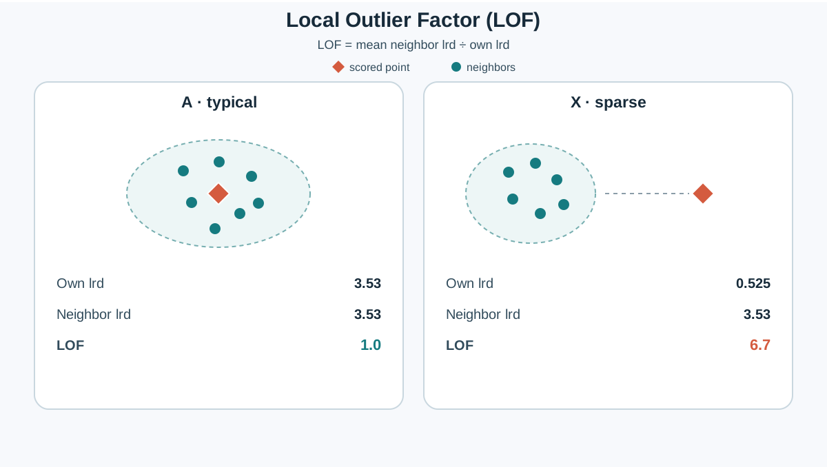
Let's make this concrete. Take a small 2D dataset with a tight cluster, a sparse cluster, and one candidate anomaly. Use k = 3.
Points (approximate layout):
- Tight cluster: A(0, 0), B(0.2, 0), C(0, 0.2), D(0.2, 0.2)
- Sparse cluster: E(5, 5), F(6, 5), G(5, 6), H(6, 6)
- Candidate: X(1.5, 1.5)
We will compute LOF for X and for A, an ordinary point in the tight cluster.
Step 1 — k-distances and neighbor sets. For each point, find the distance to its 3rd nearest neighbor.
- A's three nearest are B, C, D. Distances ≈ 0.2, 0.2, 0.283. So k-distance(A) ≈ 0.283.
- X's three nearest are D, C, B. Distances ≈ 1.84, 1.92, 1.95. So k-distance(X) ≈ 1.95.
- For the neighbors of X (D, C, B), their k-distances are all ≈ 0.283, since they sit in the tight cluster.
Step 2 — reachability distances from X to its neighbors. For each neighbor o, take the max of o's k-distance and d(X, o).
- reach-dist(X, D) = max(0.283, 1.84) = 1.84
- reach-dist(X, C) = max(0.283, 1.92) = 1.92
- reach-dist(X, B) = max(0.283, 1.95) = 1.95
Sum ≈ 5.71. With |N_k(X)| = 3, lrd(X) = 3 / 5.71 ≈ 0.525.
Step 3 — lrd for A. A's neighbors B, C, D all sit within the tight cluster, so their k-distances are ≈ 0.283 and the raw distances are ≈ 0.2. The floor dominates.
- reach-dist(A, B) = max(0.283, 0.2) = 0.283
- reach-dist(A, C) = 0.283
- reach-dist(A, D) = max(0.283, 0.283) = 0.283
Sum ≈ 0.849. lrd(A) = 3 / 0.849 ≈ 3.53.
Step 4 — LOF. For X, we need the lrd of its neighbors D, C, B. Each sits in the tight cluster, so each has lrd ≈ 3.53.
LOF(X) ≈ (3.53 + 3.53 + 3.53) / (3 · 0.525) ≈ 10.59 / 1.575 ≈ 6.7
For A, its neighbors B, C, D also have lrd ≈ 3.53, and lrd(A) ≈ 3.53.
LOF(A) ≈ (3.53 + 3.53 + 3.53) / (3 · 3.53) ≈ 1.0
The verdict is clean. A scores right at the baseline. X scores nearly seven times its neighborhood density — a strong outlier signal, even though X is not the farthest point from the origin in this dataset.
Note: Your hand calculation and a library call will diverge slightly. Tie handling, self-exclusion in the neighbor query, and the exact metric all shift the numbers. The structure of the result — X ≫ 1, A ≈ 1 — is what you are checking.
What the Score Does and Does Not Tell You
LOF flags points whose local density is lower than their neighbors'. It does not tell you whether that point is a data-entry error, a rare valid case, or the most interesting observation in your dataset. That judgment is yours.
What the score is sensitive to:
- k. Small k reacts to micro-neighborhoods and can flag noise. Large k drifts toward global density comparison and can miss local anomalies. There is no universal value; sweep a few and watch which points move.
- Scaling and metric. Everything is built on distances. Change the metric, change the ranking.
- Duplicates. They can push lrd to infinity and distort the ratio.
- Cluster size imbalance. A very small cluster can look like a cluster of outliers to a large one.
How it differs from neighbors in the same category: global distance methods compare every point to one baseline. Isolation-based methods split on feature values rather than measuring density. LOF measures density relative to a local neighborhood, which is why it handles heterogeneous density better than either.
Reach for LOF when your data has regions of genuinely different density, your dataset is moderate in size, and you want a ranked list rather than a hard label. Do not reach for it when you are working in very high dimensions, when your dataset is huge and the neighbor queries become the bottleneck, or when you need a calibrated probability rather than a ranking.
From Derivation to a Reproducible Check
The derivation is only useful if you can verify it. Here is the next move.
Recompute the worked example with a nearest-neighbors query. Pull the k-distances, compute reachability distances by hand, and compare your lrd and LOF values against a library implementation on the same data. When they disagree, the disagreement is the lesson — check tie handling, self-exclusion, and the metric.
Then vary k. Watch which points move in and out of the top-ranked list. Then rescale one feature and watch the ranking shift again. That shift is evidence that the metric, not the algorithm, is doing much of the work.
Treat the score as a ranking to investigate, not a verdict to act on. The point that looked far was not the anomaly. The point that looked close was. LOF compares a point's local reachability density to its neighbors' — and once you can compute that ratio by hand, you can trust it in code.
Knowledge check
Final check
Finish the article by checking the ideas you just learned.
References
Build stronger machine learning foundations
Use structured resources to connect theory, scikit-learn workflows, and evaluation practice.


