XGBoost’s Regularized Objective: Derive Leaf Weights and Split Gain

Two candidate splits sit in front of you. One carves the data into two clean, balanced groups. The other produces a lopsided partition that looks worse by every impurity measure you learned from decision trees. XGBoost picks the second one — or refuses to split at all. If that has ever felt like the library ignoring your intuition, the gap is not in the library. It is in the objective.

Once you see the objective, the leaf weights and the split decision stop being constants handed down by the library. They become algebra you can do on paper.

This article assumes you already know that gradient boosting adds trees sequentially and that each tree corrects the previous ensemble. If that is still fuzzy, the earlier XGBoost overview is the right place to start. Here we go one level down: the actual quantity XGBoost minimizes at each round, and what falls out of it.

What the Objective Is Actually Optimizing

At boosting round $t$, the model's prediction for sample $i$ is the running sum of all previous trees plus the new tree $f_t$:

$\hat{y}_i^{(t)} = \hat{y}_i^{(t-1)} + f_t(x_i)$

The full objective for the round is data loss plus a complexity penalty on every tree built so far:

$\text{Obj}^{(t)} = \sum_{i=1}^{n} l\left(y_i, \hat{y}_i^{(t)}\right) + \sum_{k=1}^{t} \Omega(f_k)$

The penalty is inside the objective, not bolted on afterward. That distinction is the whole article.

Because the previous trees are already fixed, only $f_t$ is free. We approximate the loss with a second-order Taylor expansion around the current prediction $\hat{y}_i^{(t-1)}$:

$\text{Obj}^{(t)} \approx \sum_{i=1}^{n} \left[ l(y_i, \hat{y}_i^{(t-1)}) + g_i f_t(x_i) + \tfrac{1}{2} h_i f_t(x_i)^2 \right] + \Omega(f_t) + \text{const}$

Here $g_i$ and $h_i$ are the first and second derivatives of the loss with respect to the current prediction, evaluated at $\hat{y}_i^{(t-1)}$:

$g_i = \partial_{\hat{y}^{(t-1)}} \, l(y_i, \hat{y}^{(t-1)}), \qquad h_i = \partial^2_{\hat{y}^{(t-1)}} \, l(y_i, \hat{y}^{(t-1)})$

Once the previous round is fixed, $g_i$ and $h_i$ are numbers, not functions. That is what makes the rest of the derivation tractable.

Drop the constant term $l(y_i, \hat{y}_i^{(t-1)})$ — it does not depend on $f_t$, so it cannot change which tree we choose. What remains is the working objective:

$\tilde{\text{Obj}}^{(t)} = \sum_{i=1}^{n} \left[ g_i f_t(x_i) + \tfrac{1}{2} h_i f_t(x_i)^2 \right] + \Omega(f_t)$

Note: This is where XGBoost diverges from generic gradient boosting. Classical gradient boosting fits the new tree to the negative gradient $-g_i$. Here we keep both $g_i$ and $h_i$, so the tree sees the local curvature of the loss, not just its slope. The approximation is only as good as the local quadratic fit — with a large learning rate or a badly initialized model, that fit is a weaker guide, which is one reason shrinkage still matters.

The Regularization Term and Why It Has Two Parts

For a tree with $T$ leaves and leaf weights $w_1, \dots, w_T$, XGBoost defines:

$\Omega(f) = \gamma T + \tfrac{1}{2} \lambda \sum_{j=1}^{T} w_j^2$

Two parameters, two jobs:

• $\gamma$ charges a flat price per leaf. Every leaf you create costs $\gamma$, whether or not it earns its keep. It is a per-split toll.
• $\lambda$ is an L2 penalty on leaf magnitude. It does not care how many leaves exist, only how loud each one is allowed to be.

I think of it as structure versus volume. $\gamma$ controls how many leaves the tree is allowed to grow. $\lambda$ controls how much any single leaf is allowed to say. The derivation below will show exactly where each one lands.

XGBoost also supports an L1 penalty on leaf weights (reg_alpha), which can drive some weights to exactly zero and induce sparsity. But L1 is non-differentiable at zero, so it needs soft-thresholding rather than the clean closed form we are about to derive. We stick to the L2 case here, and that is a deliberate choice, not an oversight.

Grouping by Leaf: From Per-Sample to Per-Leaf

A tree predicts a constant inside each leaf. So $f_t(x_i) = w_{q(x_i)}$, where $q(x_i)$ maps sample $i$ to its leaf index. Define $I_j$ as the set of training indices landing in leaf $j$, and define the per-leaf gradient and Hessian sums:

$G_j = \sum_{i \in I_j} g_i, \qquad H_j = \sum_{i \in I_j} h_i$

Substituting into the working objective turns the sum over $n$ samples into a sum over $T$ leaves:

$\tilde{\text{Obj}}^{(t)} = \sum_{j=1}^{T} \left[ G_j w_j + \tfrac{1}{2}(H_j + \lambda) w_j^2 \right] + \gamma T$

This is the step most readers skip, and then wonder why the closed form appears out of nowhere. The reorganization is the point: once the tree structure $q$ is fixed, the leaves are independent. There is no $w_1 w_2$ term. Each leaf is its own one-variable quadratic, and that independence is what makes a closed-form solution possible at all.

Picture a small tree with three leaves. Each leaf collects its own $G_j$ and $H_j$ from the samples that fall into it. The whole objective is just three separate quadratics plus a flat $\gamma T$ charge.

Deriving the Optimal Leaf Weight

Each leaf contributes a convex quadratic in $w_j$:

$\ell_j(w_j) = G_j w_j + \tfrac{1}{2}(H_j + \lambda) w_j^2$

Because $h_i \geq 0$ for convex losses and $\lambda > 0$, the coefficient on $w_j^2$ is positive, so the minimum is where the derivative is zero. No iterative search needed.

$\frac{\partial \ell_j}{\partial w_j} = G_j + (H_j + \lambda) w_j = 0$

Solving:

$w_j^{*} = -\frac{G_j}{H_j + \lambda}$

Read the formula. The numerator is the summed gradient direction. The denominator is summed curvature plus the penalty. The minus sign is there because $G_j$ points in the direction that increases loss, so the optimal step moves against it.

Why $\lambda$ in the denominator matters: it inflates the effective curvature, so the same gradient signal produces a smaller step. A leaf with a strong signal but a small $H_j$ gets damped hardest. That is the flat-region protection — leaves where the loss barely curves get pulled toward zero instead of taking a confident step on thin evidence.

Two sanity checks you can run mentally:

• As $\lambda \to 0$, the formula collapses to the Newton step $-G_j / H_j$.
• As $\lambda \to \infty$, $w_j^{*} \to 0$.

Substituting $w_j^{*}$ back into the objective gives the structural score of the tree:

$\tilde{\text{Obj}}^{*} = -\frac{1}{2} \sum_{j=1}^{T} \frac{G_j^2}{H_j + \lambda} + \gamma T$

Common mistake: The score is negative when the tree helps — a lower objective is better, and the data-loss term contributes a negative quantity. Readers often expect a positive "score" and then misread the sign of the gain. Keep the sign convention straight: negative is good.

From Structural Score to Split Gain

A split replaces one leaf with a left and a right child. The change in objective is the child score minus the parent score. Writing it out:

$\text{Gain} = \tfrac{1}{2} \left[ \frac{G_L^2}{H_L + \lambda} + \frac{G_R^2}{H_R + \lambda} - \frac{(G_L + G_R)^2}{H_L + H_R + \lambda} \right] - \gamma$

The $\gamma$ term appears once per split because the split adds exactly one leaf. That is why $\gamma$ is a hard floor rather than a soft penalty: a split is kept only when the bracketed improvement strictly exceeds $\gamma$.

The bracketed term is not guaranteed to be non-negative. It is non-negative when the split genuinely reduces the regularized objective, but a bad partition can push the child-score sum below the parent score — the split makes things worse before $\gamma$ is even applied. The worked example below shows exactly this case. So $\gamma$ does two jobs: it vetoes weak-but-positive splits, and it adds a further penalty on top of splits that were already harmful.

Two contrasts worth holding onto:

The shape of the formula is similar to impurity gain — parent minus children — but the quantity being measured is entirely different. Impurity criteria score partitions by label purity and have no notion of the current model's residuals, no Hessian weighting, and no per-leaf price. Without $h_i$, the gain reduces to a gradient-only criterion and loses the curvature weighting that makes small-$H$ leaves cautious.

A Worked Example Where Gamma Changes the Answer

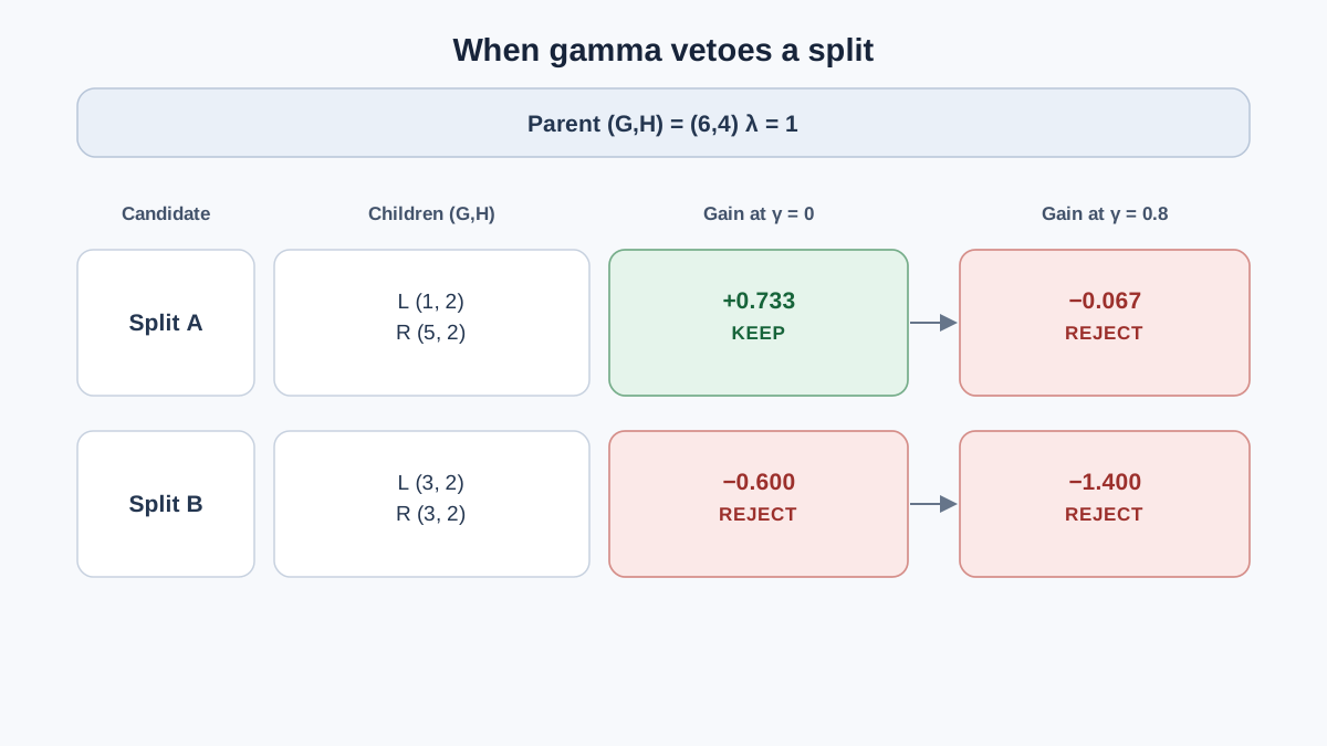
Let's make the arithmetic visible. Use squared-error loss, where $g_i = \hat{y}_i - y_i$ and $h_i = 1$ for every sample. That keeps the Hessian sums honest: $H_j$ is just the count of samples in leaf $j$.

Suppose a parent leaf has $G_P = 6$ and $H_P = 4$. Two candidate splits:

Take $\lambda = 1$. Compute the parent score first:

$\text{Parent} = \frac{G_P^2}{H_P + \lambda} = \frac{36}{5} = 7.2$

Split A:

$\frac{25}{3} + \frac{1}{3} = 8.667 \quad \Rightarrow \quad \text{Gain}_A = \tfrac{1}{2}(8.667 - 7.2) - \gamma = 0.733 - \gamma$

Split B:

$\frac{9}{3} + \frac{9}{3} = 6.0 \quad \Rightarrow \quad \text{Gain}_B = \tfrac{1}{2}(6.0 - 7.2) - \gamma = -0.6 - \gamma$

With $\gamma = 0$, split A wins with gain $0.733$ and split B is rejected outright — its bracketed term is negative, meaning the split would make the objective worse. This is the case where the L2 penalty alone kills a split.

Now raise $\gamma$ to $0.5$. Split A's gain becomes $0.233$, still positive, still kept. Raise $\gamma$ to $0.8$ and split A drops below the floor: the split is rejected even though it reduces training loss. That is $\gamma$ acting as a hard floor.

Now change $\lambda$ instead. Set $\lambda = 10$ and recompute with $\gamma = 0$:

$\text{Parent} = \frac{36}{14} = 2.571, \quad \text{Split A} = \frac{25}{12} + \frac{1}{12} = 2.167, \quad \text{Split B} = \frac{9}{12} + \frac{9}{12} = 1.5$

Split A's gain is now $\tfrac{1}{2}(2.167 - 2.571) = -0.202$. Split B's is $\tfrac{1}{2}(1.5 - 2.571) = -0.536$. Both are rejected. Under small $\lambda$, split A looked strong; under large $\lambda$, the same split loses to the penalty. $\lambda$ changes which splits clear zero, not just how large the gains are.

The arithmetic is fully visible on purpose. Reproduce it on paper before you trust it.

What This Derivation Does and Does Not Explain

This is the exact objective for the L2 case with a fixed tree structure. Real implementations add approximate split finding, histogram binning, sparsity-aware handling of missing values, and column subsampling. None of those change the algebra above, but all of them change runtime and behavior.

A positive gain is a statement about the training objective at this round, not a guarantee of better held-out performance. The regularized objective is a proxy for generalization, not a proof of it.

The second-order approximation is local. With a large learning rate or a badly initialized model, the quadratic fit is a weaker guide, and the step the formula recommends may overshoot.

$\gamma$ and $\lambda$ also interact with max_depth and min_child_weight, which are structural constraints outside $\Omega$. Tuning one while ignoring the others produces confusing results.

When this derivation is the right tool: you are writing a custom objective, debugging why a split was rejected, or reasoning about why a leaf value came out smaller than the raw gradient suggested. When it is not: routine model fitting, where the library's defaults and a validation split will teach you more per minute.

The Decision Rule to Carry Forward

When a split is rejected, check which parameter did it. If $\gamma$ vetoed the split, the bracketed improvement was real but too small to pay the toll — lower $\gamma$ if you want more structure. If $\lambda$ flattened the leaf weights, the split may have been accepted but its leaves are whispering instead of speaking — lower $\lambda$ if you want sharper leaf values. Those are different diagnoses with different fixes.

Here is the next move. Take the numbers from the worked example, change $\lambda$ by a factor of ten, and predict the new leaf weights before you compute them. If your prediction matches, the objective is yours. If it does not, the gap between prediction and computation is the lesson — and it is worth more than another read-through.