
Decision Tree Cost-Complexity Pruning: Derive the Fit–Size Tradeoff
A fully grown decision tree can score near-perfect on the data it was trained on and still lose to a single split on data it has never seen. The usual…

Key topics
A fully grown decision tree can score near-perfect on the data it was trained on and still lose to a single split on data it has never seen. The usual advice is to "just tune ccp_alpha." That advice is fine as far as it goes, but it hides the interesting part. Pruning is not cleanup you run after training. It is a second optimization problem with its own objective, its own notation, and its own blind spots. Once you can derive that objective, ccp_alpha stops being a magic knob and becomes a price you set deliberately.
If you have already worked through the intuition of pre-pruning versus post-pruning and the overfitting symptom, we can skip the taxonomy. Here we build the formal criterion, work a small comparison by hand, and then draw the boundary around what the objective can and cannot promise.
Why a Grown Tree Needs a Second Objective
A decision tree grows greedily. At each node, the algorithm picks the split that improves some local impurity measure the most, then recurses. That procedure is myopic by design: it evaluates one split at a time and has no mechanism to ask whether an entire subtree, taken as a whole, earns its keep.
This is the horizon effect. At split time you cannot tell whether one extra node will pay off three levels down, so growth decisions are made blind to the final size of the tree. The result is a tree that keeps splitting until its leaves are pure, which is another way of saying it memorizes the training set.
So we have two competing quantities:
- Fit: how well the tree classifies the training data, usually measured as error.
- Size: how many leaves the tree has, which stands in for complexity.
Pruning reframes the question as a constrained problem: minimize error subject to a budget on the number of leaves. That constraint is awkward to optimize directly, so we relax it. The Lagrangian relaxation of "minimize error subject to a size budget" produces exactly the penalty form we are about to write down. The penalty term is not arbitrary; it is the price of the constraint.
Notation: Tree, Leaves, Error, and Alpha
Before the derivation, pin down every symbol and connect it to something you can point at in a fitted tree.
- T: a subtree of the fully grown tree. Every candidate we consider is a subtree of the original, never a new tree built from scratch.
- |T|: the number of terminal nodes, or leaves, in that subtree. This is our size measure.
- R(T): the training error of subtree T. For classification this is typically the misclassification rate; for regression it is usually squared error. The choice matters, and we will come back to why.
- α (alpha): the complexity parameter, the price paid per leaf.
The cost-complexity criterion is:
The two terms can be added because they share units. R(T) is an error rate, and α is an error rate per leaf, so α |T| is also an error rate. That is the whole reason the penalty takes this shape rather than, say, multiplying error by size.
One thing worth stating plainly: α is not a hyperparameter of the tree-building algorithm. The tree is grown first, without any knowledge of α. α is a hyperparameter of the pruning objective, and it is selected outside the training fit, typically by cross-validation.
Notice the assumption baked into R(T). We are treating training error as a usable proxy for the quantity we actually care about, which is error on new data. That assumption is the crack the entire method rests on, and it is where the guarantees end.
Knowledge check
Check your understanding
Answer this question before you continue.
Deriving the Weakest Link: Which Subtree Goes First
The criterion tells you how to score a tree. It does not yet tell you which subtree to remove. Let's derive that.
Consider an internal node t with a subtree hanging below it. Compare two options: keep the subtree, or collapse t into a single leaf.
- If we collapse, the error changes by
R(leaf_t) - R(t), whereR(leaf_t)is the error of the single leaf that replaces the subtree. This quantity is the increase in error caused by collapsing — it is positive when the subtree was doing useful work. - The leaf count drops by
|t| - 1, since we remove|t|leaves and add one back.
The collapse is worth doing when the error increase per leaf removed is small. That ratio is the effective alpha of the node:
The node with the smallest effective alpha is the weakest link: it is the cheapest subtree to remove in terms of error per leaf saved. A small positive ratio means the subtree is barely earning its leaves — collapsing it costs almost nothing in fit while shrinking the tree. As α increases past a node's effective alpha, that node becomes the first candidate to prune.
Here is the consequence that makes the method cheap. Because each step only removes subtrees and never re-adds them, the sequence of optimal trees is nested. As α sweeps from 0 upward, you get a path from the fully grown tree down to the root alone, with each tree a subtree of the previous one. That nesting is what lets you compute the whole candidate sequence in one pass instead of re-optimizing from scratch at every α.
It is also a limitation. The search space is restricted to subtrees of the original greedy tree. A better small tree that the growth pass never built is simply not on the menu.
Knowledge check
Check your understanding
Answer this question before you continue.
A Worked Comparison of Two Candidate Subtrees
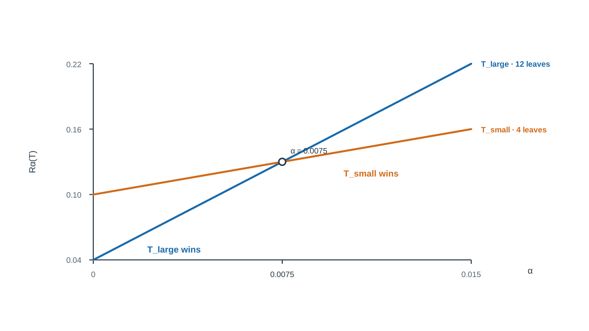
Numbers make this concrete. Suppose we have a small training set of 100 examples and two candidate subtrees.
| Subtree | Leaves | Training error R(T) | α = 0.01 penalty | α = 0.01 total | α = 0.05 penalty | α = 0.05 total |
|---|---|---|---|---|---|---|
| T_large | 12 | 0.04 | 0.12 | 0.16 | 0.60 | 0.64 |
| T_small | 4 | 0.10 | 0.04 | 0.14 | 0.20 | 0.30 |
At α = 0.01, the large tree wins: 0.16 versus 0.14 is close, but the extra leaves are cheap enough that the lower error pays for them. At α = 0.05, the smaller tree wins decisively: 0.30 versus 0.64. The penalty on twelve leaves has grown large enough to overwhelm the fit advantage.
The crossover happens where the two objectives are equal:
Below that α, the larger tree is the better choice under the criterion. Above it, the smaller tree is. Neither tree is "better" in any absolute sense. α is choosing which tradeoff you are willing to pay for, and the criterion is just doing the arithmetic.
Warning: That crossover was computed entirely on training error. The "winner" at any α is a statement about the training set, not about new data. A tree that wins the objective can still lose on held-out data.
Knowledge check
Check your understanding
Answer this question before you continue.
What the Objective Does Not Guarantee
This is the part that gets skipped, and it is the part that matters most.
The criterion never sees validation or test data. It minimizes training error plus a size penalty. It cannot optimize generalization directly, because generalization is not in the objective.
Smaller is not automatically better. If the removed subtree captured real signal, pruning increases bias and hurts held-out performance. The penalty is a proxy for complexity, not a measurement of it. Two trees with the same leaf count can differ enormously in how much they overfit.
The nested sequence restricts the candidates. You only ever choose among subtrees of the original tree. If the greedy growth pass built a poor structure, pruning can only trim it, not rebuild it.
The error term's definition matters. Misclassification rate is insensitive to how confident or how wrong a leaf's predictions are. A leaf that is 51% one class and 49% another counts the same as a leaf that is 99% one class. That insensitivity can cause the criterion to prune subtrees that were doing useful work.
The honest summary: α must be chosen by an external procedure such as cross-validation over the candidate sequence, and even then the result is a selection under uncertainty, not a proof.
Knowledge check
Check your understanding
Answer this question before you continue.
Choosing Alpha Without Fooling Yourself
The practical payoff of the derivation is that you do not search over all possible trees. You get a small, ordered set of candidates — the nested sequence — and you evaluate them.
Select α with cross-validation on training data only. The held-out set is for the final read, not for picking the penalty.
Common mistake: Tuning α against the test set. That converts the test set into a second training set and inflates the reported score. The number you get back will look better than the model actually is.
Common mistake: Reading the training-error curve as evidence of improvement. Training error can only rise as α increases, so it tells you nothing about generalization. The curve you want is the cross-validated one.
Reach for cost-complexity pruning when you want a compact, inspectable tree and you can afford a cross-validated selection step. The objective itself cannot tell you whether a pruned tree will beat an ensemble on your data — that is a separate question, answered by comparing candidates under the same validation procedure. What the criterion does give you is a principled way to narrow a single tree down to a small candidate set before you spend any evaluation budget on it.
Where to Take This Next
You now own three things: a criterion you can derive, a candidate sequence you can reason about, and a clear statement of what the objective cannot do.
The next move is to make it visible. Take a tree you have already grown, extract the candidate subtree sequence, and plot training error against α alongside a cross-validated error estimate. Watch the crossover happen in your own output rather than trusting the formula. That plot will teach you more about the fit–size tradeoff than any table of numbers, because you will see the point where the penalty starts buying you something real — and the point where it stops.
Knowledge check
Final check
Finish the article by checking the ideas you just learned.
Build stronger machine learning foundations
Use structured resources to connect theory, scikit-learn workflows, and evaluation practice.


