Gradient Boosting as Additive Function Fitting: Derive the Pseudo-Residuals

Fit the next tree to the error. That instruction works beautifully for squared loss and then quietly falls apart the moment you switch to log loss. The target you compute is no longer the error. It is something else wearing the same name.

The intuition article in this series gave you the loop: build a weak learner, correct the ensemble, repeat. This piece replaces the special case with the general rule. By the end, you will be able to write down the negative gradient of any differentiable loss and derive the boosting target yourself, instead of trusting the library to hand it to you.

The Additive Model and the Empirical Loss

Fix the object we are optimizing before touching any derivative.

An additive model builds a prediction as a sum of stagewise learners:

$F_m(x) = F_0(x) + \sum_{j=1}^{m} \nu \, h_j(x)$

Here $F_0$ is an initial constant, $h_j$ is the learner added at stage $j$, and $\nu$ is a shrinkage multiplier we will return to. The initial model is problem-specific. For least-squares regression, the conventional choice is the mean of the training targets; for binary classification with log loss, it is the log-odds of the base rate.

The empirical loss over $n$ training examples is

$L(F) = \sum_{i=1}^{n} \ell(y_i, F(x_i))$

Read that carefully. $L$ is a function of the entire prediction vector $(F(x_1), \dots, F(x_n))$, not of a finite parameter vector. There is no $\theta$ to differentiate against. The variable is the function itself.

Two constraints define the game:

• Forward stagewise. At stage $m$ we add one $h_m$ and never revisit earlier stages. No joint re-optimization.
• Restricted function class. Each $h_m$ is drawn from a class $\mathcal{H}$, usually fixed-depth regression trees. That restriction is what makes the step tractable. It is also what makes the result greedy rather than globally optimal.

State the assumptions up front, because they bound everything that follows. The per-example loss $\ell(y, F)$ must be differentiable in its second argument. The training set is finite. The class $\mathcal{H}$ is closed under the operations we apply later — specifically, we need to be able to fit a learner to arbitrary real-valued targets, which regression trees can do.

Why the Ideal Next Learner Is Intractable

The exact stagewise objective is clean to write and impossible to solve directly:

$h_m = \arg\min_{h \in \mathcal{H}} \sum_{i=1}^{n} \ell\big(y_i, \; F_{m-1}(x_i) + h(x_i)\big)$

To solve this exactly, you would enumerate every function in $\mathcal{H}$ and evaluate the total loss after adding each one. For a tree class, that means searching over every possible partition of the feature space at every depth. The search space is combinatorial and the loss surface is not convex in the tree structure.

So we cheat, but we cheat in a principled direction. Instead of solving the stagewise problem, we take a step in function space that mirrors gradient descent in parameter space. In parameter space, we cannot jump to the minimum, so we compute the gradient and move a small distance along it. In function space, we cannot enumerate $\mathcal{H}$, so we compute the steepest-descent direction and fit the best available learner to it.

Note: This is a greedy heuristic. It does not solve the stagewise problem exactly. It solves a first-order approximation of it, and the approximation is only as good as the learner class and the step size allow.

Deriving the Negative Gradient Target

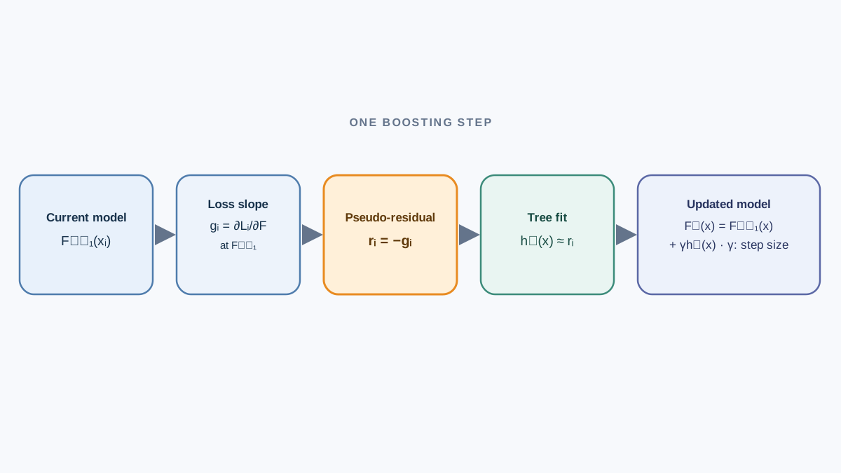
Now the derivation. It is short, and every symbol has a job.

Differentiate the empirical loss with respect to the current prediction for a single training example. Define

$g_i = \frac{\partial \, \ell(y_i, F(x_i))}{\partial F(x_i)} \bigg|_{F = F_{m-1}}$

This is the per-example gradient: how much the loss changes when you nudge the model's prediction for example $i$ by a small amount, holding every other prediction fixed.

The steepest-descent direction in function space is the negative gradient, evaluated at the current model's predictions. So the ideal next learner would satisfy

$h_m(x_i) \approx -g_i \quad \text{for each } i$

We cannot fit an arbitrary function, so we fit the best function in $\mathcal{H}$ to the values $-g_i$. Define the pseudo-residual

$r_i = -g_i = -\frac{\partial \, \ell(y_i, F(x_i))}{\partial F(x_i)} \bigg|_{F = F_{m-1}}$

and train $h_m$ as a regression model with targets $r_i$.

That is the whole trick. The "residual" label is a historical accident: for squared loss, $r_i$ happens to equal the ordinary residual. For every other loss, it is a gradient-derived quantity with different units, a different range, and a different meaning.

Convention matters here. You will see the update written as $F_m = F_{m-1} + \nu h_m$ and also as $F_m = F_{m-1} - \nu h_m$. Both are correct; they differ in whether the learner is fit to $r_i = -g_i$ (add) or to $g_i$ (subtract). Pick one and stay consistent, because mixing conventions flips the sign of your entire ensemble. The squared-loss case aligns pseudo-residuals with ordinary residuals only when the sign convention is held fixed.

One more boundary. If $\ell$ is not differentiable in the prediction — 0-1 loss is the canonical example — the derivation does not apply. You cannot take the gradient of a step function. This is why classification uses smooth surrogates like log loss or the logistic loss: they approximate the decision boundary you care about while remaining differentiable. Hinge loss is a partial exception: it is differentiable almost everywhere, but its flat regions and kink mean the gradient carries no information at some points, so the derivation applies only where the gradient is defined and nonzero.

Worked Example: Squared Loss and Log Loss

Two cases make the derivation concrete. One where pseudo-residuals are residuals, one where they visibly are not.

Squared loss

$\ell(y, F) = \tfrac{1}{2}(y - F)^2$

Differentiate with respect to $F$:

$\frac{\partial \ell}{\partial F} = -(y - F) = F - y$

The negative gradient is

$r_i = -(F(x_i) - y_i) = y_i - F(x_i)$

That is the ordinary residual. The derivation recovers the intuition exactly, under the convention that the learner is added to the ensemble.

Log loss for binary classification

Let $F$ be the log-odds score and $p = \sigma(F) = 1/(1 + e^{-F})$ the predicted probability. The per-example loss is

$\ell(y, F) = -\big[y \log p + (1 - y)\log(1 - p)\big]$

Differentiate with respect to $F$. Using $\partial p / \partial F = p(1-p)$:

$\frac{\partial \ell}{\partial F} = p - y$

The negative gradient is

$r_i = y_i - p_i$

This is a residual in probability space — the gap between the label and the predicted probability — but it is not a residual in score space. The tree is fit to values in $[0, 1]$ while the ensemble accumulates scores in $(-\infty, \infty)$. The units do not match, and that mismatch has a practical consequence: the leaf values produced by fitting to $r_i$ are not on the same scale as the raw label, so implementations refine leaf values after the tree structure is fixed.

Loss	Gradient $\partial \ell / \partial F$	Pseudo-residual $r_i$	Range of $r_i$
Squared	$F - y$	$y - F$	Same as label
Log loss	$p - y$	$y - p$	$[-1, 1]$

Same derivation, two different objects. The table is the whole point of this section.

Step Size and Line Search

Fitting $h_m$ to the pseudo-residuals gives you a direction. It does not give you a distance.

After the tree structure is fixed, solve a one-dimensional line search for the multiplier that minimizes the loss along that direction:

$\gamma_m = \arg\min_{\gamma} \sum_{i=1}^{n} \ell\big(y_i, \; F_{m-1}(x_i) + \gamma \, h_m(x_i)\big)$

For squared loss, this has a closed form: $\gamma_m$ is the least-squares coefficient of the residual on the fitted values, which reduces to a simple ratio of sums. For log loss and most other losses, there is no closed form and you solve it numerically or approximate it.

In practice, libraries do not run a full line search. They use a fixed shrinkage parameter $\nu$ — the learning rate — and often compute per-leaf optimal values instead of a single global $\gamma_m$. Shrinkage and line search are related but not identical: line search finds the best step along the direction, shrinkage deliberately takes a smaller step than optimal to leave room for later learners to correct.

The tradeoff is direct. Small steps need more learners to reach the same loss, which costs training time and memory. Large steps risk overshooting the minimum and destabilizing the ensemble, especially when the loss surface is steep near the current predictions. The learning rate and the number of estimators are coupled; tuning one without the other is guesswork.

From Derivation to the Boosting Procedure

Here is the algorithm, with each step mapped to the derivation that justifies it. The two step-size branches are kept separate, because they produce different updates.

1. Initialize $F_0(x)$ to a constant that minimizes the loss — the mean for squared loss, the log-odds for log loss. This is the starting point of the additive model.
2. Compute pseudo-residuals $r_i = -\partial \ell / \partial F(x_i)$ at the current predictions. This is the negative gradient step.
3. Fit a learner $h_m$ to the targets $r_i$ using the restricted class $\mathcal{H}$. This is the projection of the steepest-descent direction onto the available function class.
4. Choose the step size. Either solve the line search for $\gamma_m$, or fix a shrinkage parameter $\nu$. These are alternatives, not a single combined step.
5. Update the ensemble. With line search: $F_m = F_{m-1} + \gamma_m \, h_m$. With fixed shrinkage: $F_m = F_{m-1} + \nu \, h_m$. Use one branch consistently; do not mix $\gamma_m$ and $\nu$ in the same update.
6. Repeat until a stopping condition is met.

Implementations diverge from this textbook version in three places worth knowing. XGBoost and similar libraries use a second-order Taylor approximation of the loss, replacing the gradient-only step with a Newton step that uses both gradient and Hessian. They compute per-leaf optimal values rather than a single global step size. And they add explicit regularization terms on leaf weights and tree complexity. None of these change the core derivation; they refine the step.

For stopping, validation-based early stopping is the honest choice. Training loss decreases monotonically as you add learners, so it cannot tell you when to stop. A held-out set can.

When Pseudo-Residuals Are Not Residuals

This is the section that prevents the most expensive debugging mistakes.

Pseudo-residuals equal ordinary residuals only for squared loss under a consistent sign convention. For every other loss, they are gradient-derived targets with different units and ranges. Three consequences follow.

Debugging. A shrinking pseudo-residual magnitude does not mean the model is fitting the label better in the original units. For log loss, $r_i = y_i - p_i$ is bounded in $[-1, 1]$ regardless of how wrong the score is. A model can have small pseudo-residuals and still produce badly calibrated probabilities.

Loss choice. Switching loss changes the target distribution. Tree depth and learning rate tuned for squared loss may not transfer to log loss, because the targets have different variance, different scale, and different sensitivity to outliers. Re-tune when you switch.

Assumption boundary. The derivation requires differentiability and a function class rich enough to approximate the gradient direction. When $\mathcal{H}$ is too weak — trees that are too shallow, or a linear class on a nonlinear problem — boosting stalls regardless of iteration count. Adding more learners to a class that cannot represent the gradient direction just accumulates the same correction over and over.

Common mistake: Treating pseudo-residuals as "the error" and expecting them to shrink toward zero in the label's units. They shrink toward zero in the gradient's units, which is a different thing.

What to Do Next

The derivation is a decision rule, not a ritual. When you can write down $-\partial \ell / \partial F$ for your loss, you can derive the boosting target yourself and stop treating the library as a black box. When you cannot — because the loss is non-differentiable, or the function class cannot represent the gradient direction — the derivation stops being the right tool, and you need a different approach.

The practical next step is to run a boosting experiment and watch how learning rate and tree depth interact with the derived update. Fit a model with a small learning rate and many estimators, then a large learning rate and few. Compare the validation curves. The shape of those curves is the line search and the shrinkage parameter doing their work in the open.