How the SVM Dual Makes Kernel Substitution Possible

The primal SVM asks for a weight vector in feature space. The trained model never hands you one. It hands you a sum over training points instead — and that quiet substitution is what makes kernels legal.

This article traces that swap. We will write the soft-margin primal, introduce Lagrange multipliers, eliminate $w$ and $b$, and land on a dual objective where every training point appears only inside a pairwise inner product. Then we will replace that inner product with a valid kernel and be precise about what the replacement buys and what it does not.

If the margin geometry still feels shaky, the maximum-margin derivation is the prerequisite. Here we assume you accept that the margin is $\tfrac{2}{\|w\|}$ and that only the closest points constrain the boundary.

Why the Primal Form Hides the Kernel

Fix notation once. Training pairs are $(x_i, y_i)$ for $i = 1, \dots, n$, with $y_i \in \{-1, +1\}$. A feature map $\phi$ sends each input into a feature space, $w$ is the weight vector in that space, $b$ is the bias, $\xi_i \ge 0$ are slack variables, and $C > 0$ is the penalty on slack.

The soft-margin primal is

subject to

The assumptions matter because the dual derivation depends on all of them: the objective is convex and quadratic, the constraints are linear in $(w, b, \xi)$, the feature space may be finite-dimensional or only implicitly defined, and the margin constraints are the only place where different training points interact.

That last assumption is the one to watch. Look at the objective: $\tfrac{1}{2}\|w\|^2$ involves $w$ alone, and $C\sum \xi_i$ involves slacks alone. The data enters only through the constraints, and each constraint touches exactly one point. Nothing in the primal couples $x_i$ to $x_j$.

Now look at the structural problem. The solution is a vector $w$ in feature space. To use it, you need its coordinates, and those coordinates are defined through $\phi(x_i)$. If $\phi$ maps into a space with thousands of dimensions — or infinitely many — you cannot write $w$ down. The primal is honest about this: it asks for an object you may not be able to represent.

The Lagrangian Step That Moves Data Into the Objective

Introduce a Lagrange multiplier $\alpha_i \ge 0$ for each margin constraint and $\mu_i \ge 0$ for each non-negativity constraint on the slack. The Lagrangian is

Stationarity with respect to $w$ gives the first key relation:

This is already a shift in kind. The optimal weight vector is not an arbitrary point in feature space; it is a weighted sum of the training points' images. Stationarity with respect to $b$ gives

And stationarity with respect to $\xi_i$ gives $C - \alpha_i - \mu_i = 0$, which, combined with $\mu_i \ge 0$, yields the box constraint $0 \le \alpha_i \le C$.

Now substitute $w = \sum_i \alpha_i y_i \phi(x_i)$ back into the Lagrangian. The $\|w\|^2$ term becomes

The linear terms in $w$ cancel against the corresponding part of the constraint sum, the $b$ terms vanish because $\sum_i \alpha_i y_i = 0$, and the slack terms collapse to $C\sum_i \xi_i - \sum_i \alpha_i \xi_i - \sum_i \mu_i \xi_i = 0$. What remains is the dual:

subject to

The KKT conditions tell you which points matter. Complementary slackness requires $\alpha_i \big[y_i(w^\top \phi(x_i) + b) - 1 + \xi_i\big] = 0$. For a point strictly outside the margin with no slack, the bracket is positive, so $\alpha_i = 0$. Only points on or inside the margin — the support vectors — carry nonzero weight. The dual is sparse in a way the primal never advertised.

The Inner Product Is the Only Door the Data Walks Through

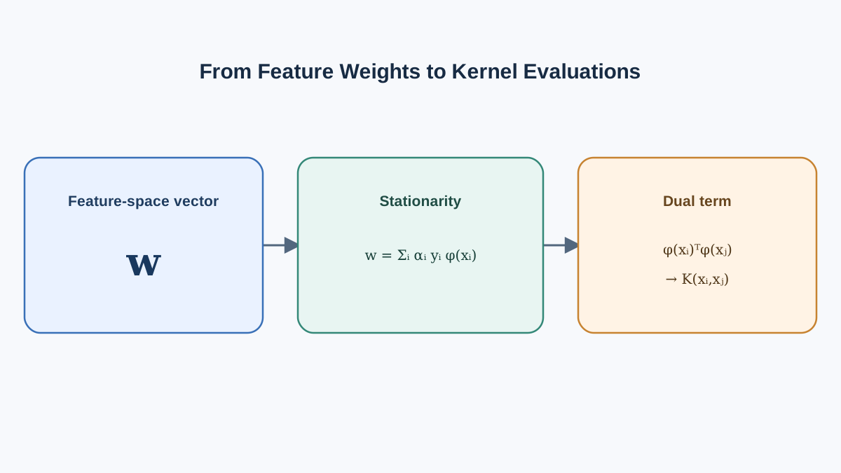
Read the dual objective again and notice what happened to $\phi(x_i)$. It never appears alone. It appears only as $\phi(x_i)^\top \phi(x_j)$ — a pairwise inner product.

The decision function inherits the same structure. Since $w = \sum_i \alpha_i y_i \phi(x_i)$, the prediction for a new input $x$ is

where the sum runs over support vectors in practice. Again, the only thing touching the data is an inner product between two examples.

This is the structural observation the whole trick rests on. The algorithm does not need the coordinates of any point. It needs a number that says how similar two points are after mapping. Contrast that with the primal, where $w$ is an explicit vector and its coordinates are the object being optimized.

Note: The dual is not merely a reformulation for convenience. It changes what the algorithm is allowed to ask for. The primal asks for coordinates. The dual asks for similarities.

Substituting a Valid Kernel

Define a kernel as a function $K(x_i, x_j)$ that returns the inner product of the images of two inputs under some feature map:

The validity condition is the part people skip. Not every symmetric similarity function is a kernel. $K$ is valid when it corresponds to an inner product in some feature space, which is equivalent to requiring that the Gram matrix $G_{ij} = K(x_i, x_j)$ be positive semidefinite for every finite set of inputs. This is the Mercer-style condition, and it is what keeps the dual a convex quadratic program.

The substitution is mechanical. Replace every occurrence of $\phi(x_i)^\top \phi(x_j)$ in the dual objective and in the decision function with $K(x_i, x_j)$:

subject to $\sum_i \alpha_i y_i = 0$ and $0 \le \alpha_i \le C$, with prediction

A Worked Example: The Degree-2 Polynomial Kernel

Take two-dimensional inputs $x = (x_1, x_2)$ and $z = (z_1, z_2)$, and consider

Expand by hand:

Now define the feature map

Then

The identity holds exactly. The kernel computes a three-dimensional inner product using only two-dimensional arithmetic. For a degree-$d$ polynomial on $m$ features, the explicit feature space has on the order of $m^d$ dimensions; the kernel evaluates in $O(m)$.

The RBF kernel, $K(x, z) = \exp(-\gamma \|x - z\|^2)$, pushes this further. Its feature space is infinite-dimensional. There is no explicit $\phi$ to write down — not expensive, impossible. The kernel is the only way in.

Warning: A function that looks like a similarity is not automatically a valid kernel. An indefinite Gram matrix can make the dual non-convex and break the optimizer, often silently, producing a model that fits nothing well.

What Kernel Substitution Buys You, and What It Does Not

What it enables: a linear separator in an implicit feature space, which corresponds to a nonlinear boundary in the input space, without ever computing $\phi$. The optimization problem is the same shape as before. Only the similarity function changed.

What it does not guarantee:

• Separability. A kernel does not make every dataset separable. It changes the space in which you look for a separator; it does not promise one exists.
• Free tuning. $C$ and the kernel hyperparameters still need to be chosen, and the wrong choices produce worse models than a plain linear fit.
• Immunity to overfitting. A flexible kernel can bend the boundary around noise as easily as around structure.

The cost structure is the practical constraint. The dual objective sums over all pairs $(i, j)$, so forming the Gram matrix is $O(n^2)$ in time and memory. That quadratic wall, not the mathematics, is why kernel SVMs stall on large datasets.

Interpretability pays a price too. The boundary is defined through similarities to support vectors, so the implicit feature space is not directly readable. You can inspect which points are support vectors; you cannot read off a coefficient per original feature.

The escape hatch for large data is an approximate explicit feature map. If you can approximate the kernel with a finite-dimensional mapping, a linear solver can do the work, and linear solvers scale. The tradeoff is approximation error, so compare against the exact kernel when you can.

My decision rule: reach for a kernel when the dataset is medium-sized, the boundary is genuinely nonlinear, and you can afford to tune. Prefer explicit features or a linear model when $n$ is large or when you need to explain the boundary.

Reading the Dual in Practice

The dual variables become visible the moment you fit a model. In scikit-learn, SVC exposes dual_coef_ and support_vectors_. Most $\alpha_i$ are zero; the nonzero ones mark support vectors. Points with $\alpha_i = C$ sit inside the margin or on the wrong side of it.

from sklearn.svm import SVC

clf = SVC(kernel="rbf", C=1.0, gamma="scale")
clf.fit(X_train, y_train)

print(clf.support_vectors_.shape[0], "support vectors out of", len(X_train))

The library is solving this dual, or an equivalent formulation, not the primal. When you pass kernel="rbf", you are handing it the similarity function that replaces the inner product.

The same dual structure reappears in kernel ridge regression and Gaussian processes. Once you see the pattern — eliminate the weights, express everything as pairwise similarities, substitute a valid kernel — you have a reusable template, not an SVM-only trick.

One diagnostic habit worth building: track the fraction of training points that end up as support vectors, but treat it as a clue rather than a verdict. A high fraction can reflect a boundary that is bending hard, but it can also reflect genuine class overlap, a representation that does not separate the classes, or a kernel whose parameters are mismatched to the data. The count tells you where to look; it does not tell you what is wrong. Pair it with held-out performance and validation behavior before you touch C or gamma. If validation error is climbing while training error keeps falling, the flexibility is the problem. If both are high, the kernel or the features may simply be a poor fit.

Where to Go Next

The chain is short enough to hold in your head: primal in terms of $w$, Lagrangian elimination, dual in terms of inner products, substitution of a valid kernel. The kernel trick is not a separate algorithm bolted onto the SVM. It is a consequence of the dual never needing coordinates.

Take a small two-dimensional dataset — two interleaved moons work well — fit an RBF kernel SVM, and plot the support vectors. Then vary gamma and watch the boundary tighten or relax. The dual variables you derived are the points you are looking at.