Derive AdaBoost’s Weight Updates From Exponential Loss

AdaBoost's algorithm listing looks like three separate rules stitched together: fit a weak learner, compute a coefficient, multiply the sample weights by an exponential. Read the listing alone and you would reasonably assume someone tuned each step independently.

They did not. All three lines are the same objective read at three different moments. Once you see the objective, the coefficient and the weight update stop being conventions you memorize and become consequences you can reproduce on a blank page.

This is the derivation. We will fix notation, justify the loss, minimize it twice, and then find the boundary where the whole additive story stops being useful.

Why AdaBoost's Rules Look Arbitrary

The weak model says "hard examples get more weight." That explains the direction of reweighting. It says nothing about the magnitude. Why multiply by $e^{\alpha_t}$ and not $1 + \alpha_t$? Why is the learner coefficient $\tfrac{1}{2}\ln\frac{1-\text{err}}{\text{err}}$ and not just $1 - \text{err}$?

The stronger model: AdaBoost is forward stagewise additive modeling under one fixed loss. At each round you add one new term to an additive score and choose that term to reduce the loss as much as possible given everything already added. The reweighting rule, the coefficient, and the final vote are not three decisions. They are three views of one partial minimization.

If you have seen boosting as sequential error correction, this is the next question: which objective makes AdaBoost's specific numbers inevitable? The answer is exponential loss, and the rest of this article is the proof.

Notation: Labels, Weak Learners, and the Additive Score

Fix every symbol before we use it.

Binary labels $y_i \in \{-1, +1\}$. The sign convention is load-bearing. It lets us write "correct" and "incorrect" as a single product $y_i h(x_i)$, which is $+1$ when the learner agrees with the label and $-1$ when it does not. That product is the margin, and margins are what the loss actually sees.

Weak learners $h_t: \mathcal{X} \to \{-1, +1\}$. Each round produces one such learner. The weak learning assumption is that $h_t$ achieves a weighted error strictly better than chance — an edge, not a miracle.

The additive score after $T$ rounds:

$F_T(x) = \sum_{t=1}^{T} \alpha_t h_t(x).$

The sign of $F_T(x)$ is the prediction. The magnitude is confidence. A large positive score means the ensemble is confidently positive.

Exponential loss over the training set:

$L = \sum_{i=1}^{N} \exp\!\big(-y_i F(x_i)\big).$

Define the margin $m_i = y_i F(x_i)$. Then the loss is $\sum_i e^{-m_i}$: a function of margin alone. Positive margins shrink the loss toward zero; negative margins blow it up. The loss never reaches zero, unlike 0/1 loss — it just gets small.

Normalized sample weights at round $t$:

$w_i^{(t)} \propto \exp\!\big(-y_i F_{t-1}(x_i)\big).$

Note the proportionality, not equality. The weights are the per-example loss terms from the previous round, rescaled to sum to one. Normalization is a convenience for computing weighted error rates; it does not change which examples the next learner cares about.

Note: The proportionality is the whole trick. If the weights were defined as equal to the exponentials, they would grow without bound across rounds and the weighted error rate would be meaningless. Normalizing keeps the quantity interpretable as a distribution over examples.

The Objective: Exponential Loss as a Margin Penalty

Why this loss and not another?

Exponential loss penalizes negative margins steeply and positive margins mildly. A confidently wrong point with margin $-3$ contributes $e^{3} \approx 20$. A confidently right point with margin $+3$ contributes $e^{-3} \approx 0.05$. The asymmetry is the point: the loss is far more interested in fixing mistakes than in rewarding correct answers.

Compare with log loss, $\log(1 + e^{-m})$. Both are convex, both are margin-based, both approach zero for large positive margins. But exponential loss grows exponentially on the negative side, while log loss grows linearly. That difference is why exponential loss is less forgiving of confidently wrong points — and why it is less robust to label noise.

Three assumptions carry the derivation:

1. Binary labels $y_i \in \{-1, +1\}$.
2. Base learners output values in $\{-1, +1\}$ — not probabilities, not real scores.
3. Weighted error strictly below $1/2$ at each round. The weak learning assumption, stated as a hard constraint.

The multiplicative structure matters too. Because $F_T = F_{T-1} + \alpha_T h_T$, the exponential of a sum becomes a product of per-round factors:

$\exp\!\big(-y_i F_T(x_i)\big) = \exp\!\big(-y_i F_{T-1}(x_i)\big) \cdot \exp\!\big(-\alpha_T y_i h_T(x_i)\big).$

That factorization is what makes sequential reweighting possible at all. Each round's loss is the previous round's loss, multiplied by one new factor per example.

Warning: The derivation below is exact only for the $\{-1, +1\}$ output convention. Real-valued or probabilistic base learners require a different coefficient — the same loss, but a different minimization over the learner's output range.

Deriving the Learner Coefficient $\alpha_t$

We are at round $t$. The score so far is $F_{t-1}$. We add one new term $\alpha_t h_t$ and ask: what value of $\alpha_t$ minimizes the loss?

Write the loss after adding the new term:

$L_t = \sum_{i=1}^{N} w_i^{(t)} \exp\!\big(-\alpha_t y_i h_t(x_i)\big),$

where $w_i^{(t)} = \exp(-y_i F_{t-1}(x_i))$ absorbs everything from previous rounds. This is the key move: the previous score is frozen, and the only free variable is $\alpha_t$.

Now split the sum. For each example, $y_i h_t(x_i)$ is either $+1$ (correct) or $-1$ (incorrect). So:

$L_t = e^{-\alpha_t} \sum_{y_i = h_t(x_i)} w_i^{(t)} + e^{\alpha_t} \sum_{y_i \neq h_t(x_i)} w_i^{(t)}.$

Let $W = \sum_i w_i^{(t)}$ be the total weight and $\text{err}_t = \frac{1}{W}\sum_{y_i \neq h_t(x_i)} w_i^{(t)}$ be the weighted error rate. Then the correctly classified mass is $W(1 - \text{err}_t)$ and the misclassified mass is $W \cdot \text{err}_t$:

$L_t = W\Big[e^{-\alpha_t}(1 - \text{err}_t) + e^{\alpha_t}\,\text{err}_t\Big].$

Differentiate with respect to $\alpha_t$ and set to zero:

$\frac{dL_t}{d\alpha_t} = W\Big[-e^{-\alpha_t}(1 - \text{err}_t) + e^{\alpha_t}\,\text{err}_t\Big] = 0.$

Solve:

$e^{\alpha_t}\,\text{err}_t = e^{-\alpha_t}(1 - \text{err}_t)$ $e^{2\alpha_t} = \frac{1 - \text{err}_t}{\text{err}_t}$ $\alpha_t = \frac{1}{2}\ln\!\left(\frac{1 - \text{err}_t}{\text{err}_t}\right).$

That is the AdaBoost learner coefficient, derived rather than declared.

Read the shape. At $\text{err}_t = 1/2$, the ratio is $1$ and $\alpha_t = 0$: a learner no better than chance gets no vote. As $\text{err}_t \to 0$, the ratio blows up and $\alpha_t$ grows large: a strong learner gets a loud voice. Above $\text{err}_t = 1/2$, the ratio drops below $1$, the log goes negative, and $\alpha_t$ turns negative — the learner is worse than chance and the ensemble would need to invert it.

Common mistake: Treating $\alpha_t = \frac{1}{2}\ln\frac{1-\text{err}}{\text{err}}$ as a formula to plug in without checking its domain. At $\text{err}_t = 0$ the coefficient diverges; at $\text{err}_t \geq 1/2$ it is non-positive and the additive interpretation collapses. The formula assumes $0 < \text{err}_t < 1/2$.

Deriving the Sample Weight Update

Now the second minimization. The weights for the next round are defined by the new score:

$w_i^{(t+1)} \propto \exp\!\big(-y_i F_t(x_i)\big) = \exp\!\big(-y_i (F_{t-1}(x_i) + \alpha_t h_t(x_i))\big).$

Factor out the previous round's score:

$w_i^{(t+1)} \propto \underbrace{\exp\!\big(-y_i F_{t-1}(x_i)\big)}_{w_i^{(t)}} \cdot \exp\!\big(-\alpha_t y_i h_t(x_i)\big).$

So:

$w_i^{(t+1)} \propto w_i^{(t)} \exp\!\big(-\alpha_t y_i h_t(x_i)\big).$

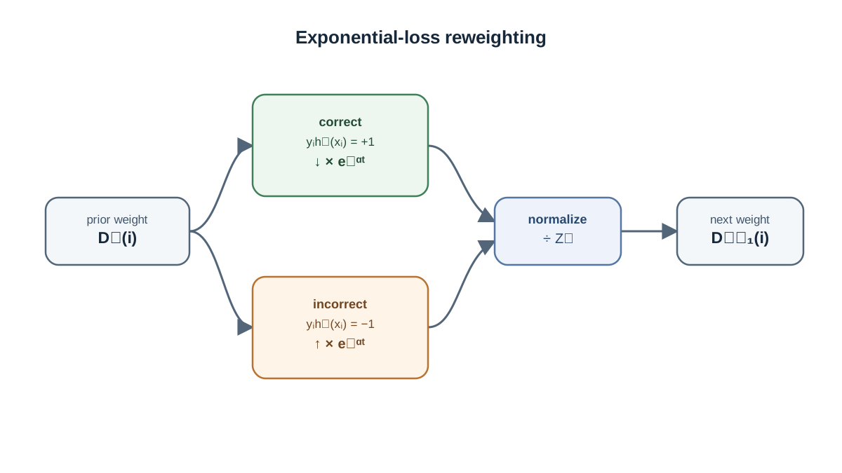
That is the reweighting rule, derived from the same loss. Now rewrite it in the familiar multiplicative form. When the example is correct, $y_i h_t(x_i) = +1$ and the factor is $e^{-\alpha_t}$. When it is wrong, $y_i h_t(x_i) = -1$ and the factor is $e^{+\alpha_t}$:

$w_i^{(t+1)} \propto \begin{cases} w_i^{(t)} e^{-\alpha_t} & \text{if correct} \\ w_i^{(t)} e^{+\alpha_t} & \text{if incorrect} \end{cases}$

Correct examples are scaled down by $e^{-\alpha_t}$; incorrect examples are scaled up by $e^{\alpha_t}$. Since $e^{\alpha_t} > e^{-\alpha_t}$ for any $\alpha_t > 0$, the misclassified examples gain relative weight.

Here is the part the derivation glosses over. The constant factor $e^{-\alpha_t}$ appears in every example's update — correct and incorrect alike. Under normalization, a uniform factor cancels. That is why the practical update only needs the misclassified examples scaled up by $e^{2\alpha_t}$ relative to the rest. The clean form is a normalization artifact, not a separate rule.

And the mechanism closes: the next learner sees a reweighted problem whose weighted error is exactly the quantity $\alpha_{t+1}$ will be computed from. The loss, the coefficient, and the weights are one loop.

A Worked Numerical Step

Let us run one round by hand. Eight labeled points, current weights uniform at $1/8$ each. The weak learner $h_t$ misclassifies three of them.

Weighted error:

$\text{err}_t = \frac{3 \cdot (1/8)}{8 \cdot (1/8)} = \frac{3}{8} = 0.375.$

Learner coefficient:

$\alpha_t = \frac{1}{2}\ln\!\left(\frac{1 - 0.375}{0.375}\right) = \frac{1}{2}\ln\!\left(\frac{0.625}{0.375}\right) = \frac{1}{2}\ln(1.667) \approx 0.255.$

Now apply the multiplicative update. Correct examples: multiply by $e^{-0.255} \approx 0.775$. Incorrect examples: multiply by $e^{+0.255} \approx 1.291$.

The raw updated weights sum to $5(0.0969) + 3(0.1614) = 0.9687$. Normalizing by dividing each by $0.9687$ gives the final column. The misclassified examples now carry $0.178$ each instead of $0.125$ — a $42\%$ relative increase in influence.

Verify the loss decreased. Before the round, with $F_{t-1}$ giving each example margin $0$: $L = 8 \cdot e^{0} = 8$. After adding $\alpha_t h_t$, correct examples have margin $+0.255$ and incorrect have margin $-0.255$:

$L' = 5 e^{-0.255} + 3 e^{0.255} \approx 5(0.775) + 3(1.291) \approx 7.75.$

The loss dropped from $8$ to $7.75$. Monotone decrease, as the derivation guarantees.

Common mistake: Forgetting to normalize. If you skip it, the next round's weighted error is computed against weights that no longer sum to one, and $\alpha_{t+1}$ silently drifts. The arithmetic looks fine; the coefficient is wrong.

One round is not convergence. The loss decreases monotonically, but what governs test behavior is the margin distribution across examples, not the aggregate loss value.

What the Derivation Assumes, and Where It Breaks

The derivation is clean. The boundaries are not.

Greedy, not global. $\alpha_t$ is optimal given $F_{t-1}$ and the chosen $h_t$. It is not the globally optimal coefficient for the final ensemble. AdaBoost is coordinate descent on the exponential loss — each round optimizes one coordinate, and the sequence converges to a minimum, but no single round sees the whole landscape.

The $\{-1, +1\}$ convention is load-bearing. Real-valued base learners need a different coefficient. The loss is the same; the minimization over a continuous output range produces a different closed form.

The weak learning assumption is not decoration. If $\text{err}_t$ stays at or above $1/2$, $\alpha_t$ turns non-positive and the additive interpretation collapses. The algorithm has no mechanism to recover from a learner that is consistently worse than chance.

Label noise is the sharp failure mode. Exponential loss grows without bound on confidently wrong points. A mislabeled example that the ensemble confidently misclassifies accumulates weight mass round after round and can dominate later learners. This is why exponential loss is less robust than log loss — the loss function's steepness on negative margins is exactly what makes it fragile to noise.

Monotone loss decrease is proven; generalization is not. The update guarantees $L_t < L_{t-1}$. It says nothing about test error. Those are separate questions, and conflating them is a common source of confusion.

Reading AdaBoost as One Objective, Not Three Rules

One loss. One additive form. Two partial minimizations. Three algorithm lines.

The chain: exponential loss defines the objective. The additive score defines the model. Minimizing over $\alpha_t$ gives the learner coefficient. Minimizing over the score gives the weight update. The final vote is just the sign of the accumulated score.

The practical consequence is that the coefficient and the weights are coupled. Change the loss and both change at once. This is why AdaBoost variants differ in their loss function, not in their reweighting tricks — the reweighting is a consequence of the loss, not an independent design choice.

When the exponential-loss view is the right lens: binary problems, reasonably clean labels, and a need to reason about margins. When it is the wrong lens: noisy labels, probabilistic outputs, or multiclass settings where a different loss and a different weighting scheme apply.

If you have already worked through gradient boosting's pseudo-residual derivation, you have seen the same additive skeleton with a different loss and a different per-learner target. AdaBoost is the special case where the loss is exponential and the target collapses to a reweighted classification problem.

Here is the next move I would take: instrument a small AdaBoost run to log $\text{err}_t$ and $\alpha_t$ at every round. Plot them. You should see $\alpha_t$ rise as $\text{err}_t$ falls, and the weight mass migrate toward the examples the ensemble keeps missing. When the curve stops matching the formula's prediction, you have found the boundary where the assumptions fail — and that is where the real learning starts.