
Split Conformal Prediction: Derive the Rank-Based Coverage Guarantee
A prediction interval built from a model's own residuals has no guarantee at all. Split conformal prediction replaces that hope with a finite-sample…

Key topics
A prediction interval built from a model's own residuals has no guarantee at all. Split conformal prediction replaces that hope with a finite-sample promise — and the promise comes from counting ranks, not from fitting a distribution.
Why Naive Residual Intervals Have No Guarantee
Suppose you fit a regression model, compute residuals on the training set, and build an interval of the form , where is the standard deviation of those residuals. This is the most common way to attach uncertainty to a prediction, and it is quietly broken in two places.
First, the residuals are optimistically small. The model was fit to minimize error on exactly those points, so the spread you measure is the spread the model has already absorbed. When the model overfits, training residuals shrink toward zero while test errors stay large. Your interval narrows precisely when it should widen.
Second, even if you compute residuals on held-out data, you are still assuming the residual distribution has a known shape. The Gaussian multiplier is a claim about the tails of a distribution you have not verified. If the true errors are heavier-tailed, the interval undercovers, and a single test set will not reliably tell you by how much.
State the goal precisely. For a fresh input and its unseen label , you want a set such that
for a chosen miscoverage level , with no distributional assumption on the data. Coverage here is a frequency statement: across repeated draws of calibration data and test points, the interval contains the label at least of the time. It is not a per-point certainty, and it is not a statement about any single prediction you happen to be looking at.
Split conformal prediction delivers exactly this. The rest of this article derives why.
Notation, the Nonconformity Score, and Exchangeability
Before the derivation, fix the objects it operates on.
Split your labeled data into two disjoint parts: a proper training set and a calibration set of size . Fit any predictor on — a linear model, a gradient-boosted tree, a neural network, it does not matter for the guarantee.
Define a nonconformity score that measures how badly a candidate label agrees with the prediction at . For regression the canonical choice is the absolute residual:
A small score means the label looks plausible; a large score means it looks like an outlier relative to the model.
Compute the calibration scores for each , and let be the score of a fresh test point. The interval will be built by comparing against the calibration scores.
Now the one assumption everything rests on.
Exchangeability: the joint distribution of is invariant to permutation. Any reordering of the points is equally likely.
Independent and identically distributed data is exchangeable, but exchangeability is the weaker and more honest condition: it does not require independence, only that no point is privileged by position. This is the load-bearing assumption. It implies that the test score is statistically indistinguishable from the calibration scores — it is not systematically larger or smaller, and its rank among the pooled scores is uniformly distributed over .
That uniformity is the entire engine of the guarantee. It holds no matter what is, no matter how wrong the model is, and no matter what the true residual distribution looks like.
It also draws a hard boundary. Time series with lagged features, spatial data with neighborhood dependence, and any setting where the distribution drifts between calibration and deployment all break exchangeability. The guarantee is stated for a fresh exchangeable point, and it silently fails outside that regime.
Knowledge check
Check your understanding
Answer this question before you continue.
The Rank Argument: Why the Quantile Is ceil((n+1)(1-alpha))
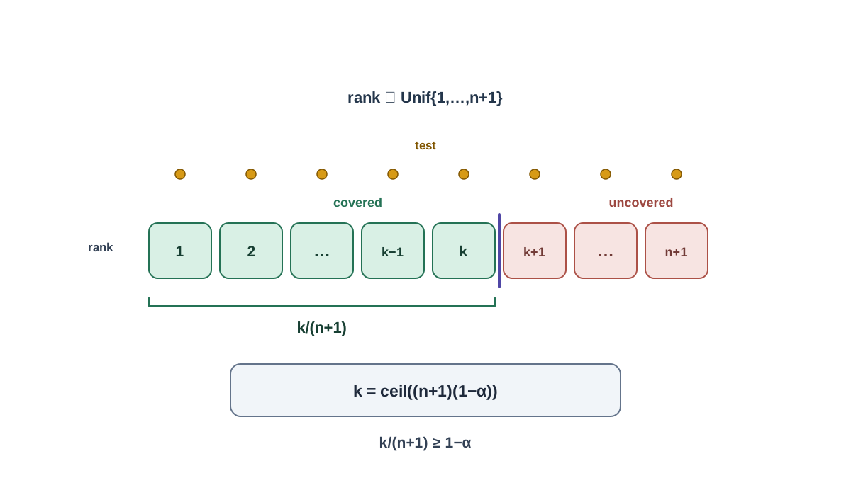
With exchangeability in hand, the threshold falls out of a counting argument.
Order the calibration scores from smallest to largest:
Pick an integer and define as the -th smallest calibration score, . The prediction interval is then
The only open question is which to use.
Pool the calibration scores with the test score to get values. Under exchangeability, is equally likely to occupy any of the ranks in this pooled set — there is nothing that makes the test point special. So for any between and ,
Now connect rank to coverage. The test point is covered exactly when , which happens exactly when the test score's rank is at most . Therefore
To hit the target , choose the smallest that keeps at or above :
This gives the coverage guarantee
The ceiling is why the guarantee is conservative rather than exact. Because must be an integer, can overshoot whenever the target rank is not itself an integer. When it is an integer, the ceiling does nothing and coverage lands exactly on target. So the overshoot is not a permanent tax — it appears only when the arithmetic forces a rounding step, and it shrinks as grows.
One caveat worth naming. With continuous scores, ties have probability zero and the rank argument is clean. With discrete or heavily tied scores — say, a model that outputs integers — several points can share a rank. The standard threshold rule still yields a valid interval: coverage is at least , and ties can only make the interval wider, never narrower. What changes is the exact equality ; the guarantee becomes an inequality. If you want the exact rank-counting statement back, break ties with a fixed convention and accept that the realized coverage may sit slightly above the nominal level. Adding noise to continuous-ize the scores is one way to do that, but it is a modeling choice, not a requirement of the method.
Knowledge check
Check your understanding
Answer this question before you continue.
Worked Example: Coverage Bound on a Small Calibration Set
Numbers make the finite-sample behavior concrete.
Take calibration points and , targeting 90% coverage. Then
So is the 90th smallest calibration score, and the interval is . The guaranteed coverage is — exactly on target here, because is an integer and the ceiling is inert.
Now shrink the calibration set. With and , , giving coverage . Still exact, for the same reason. But with and , . Since , the 6th smallest calibration score does not exist — is effectively , and the interval is the entire real line. A vacuous guarantee is still a guarantee.
The exact feasibility condition is . Substituting the definition of :
For , this holds at but fails at . The boundary sits where crosses , which gives the approximate rule — but treat that as a rough guide, not the test. The test is always . For 90% coverage, already works; for 99% coverage, you need roughly 100 calibration points before the interval stops being the whole line.
Calibration size also trades directly against sharpness. As grows, converges toward the true quantile of the residual distribution, so the interval tightens. Small calibration sets buy you a valid but wide interval; large ones buy you a valid and useful one.
Knowledge check
Check your understanding
Answer this question before you continue.
What the Guarantee Actually Promises — and What It Does Not
The most common misreading of the coverage statement is to treat it as a per-point promise. It is not.
The guarantee is marginal. It averages over the draw of the calibration set and over the draw of the test point. It says: if you repeat the whole procedure many times, the fraction of covered test points is at least . It does not say that any particular input gets a chance of coverage.
On heteroscedastic data this distinction bites hard. A single global is one number applied everywhere. In low-noise regions of the input space, the interval over-covers — it is wider than it needs to be. In high-noise regions, it under-covers. The average still hits the target, because the two errors cancel. But if your application lives in the high-noise region, you are getting less coverage than you think.
This is not a defect you can patch with a better implementation. Strong conditional coverage — a per-input guarantee — is generally unattainable in finite samples without additional structure on the problem. The marginal guarantee is what is available distribution-free, and it is worth having.
Two properties are worth keeping straight:
| Property | Split conformal prediction |
|---|---|
| Distributional assumptions | None beyond exchangeability |
| Model assumptions | None — works with any fitted predictor |
| Guarantee type | Marginal, finite-sample |
| Conditional coverage | Not guaranteed |
| Behavior with a bad model | Still covers; intervals just get wider |
That last row is the quiet strength of the method. The score is calibrated, not the model. A badly misspecified predictor produces large residuals, which produce a large , which produces wide intervals that still cover. You lose sharpness, not validity. The interval is only as informative as the score function you chose.
Knowledge check
Check your understanding
Answer this question before you continue.
When Exchangeability Breaks: Distribution Shift and Dependence
The rank-uniformity argument is a statement about a symmetric joint distribution. Remove the symmetry and the argument collapses — usually without any warning signal in your metrics.
Under covariate shift, label shift, or concept drift, the test point is no longer exchangeable with the calibration points. Its score is systematically larger or smaller, its rank is no longer uniform, and empirical coverage can fall below while every diagnostic you are watching looks fine.
Time series and spatial data are the canonical violations. If you predict from lagged features , the points are dependent by construction, and a random train/calibration split is not an exchangeable split. The same holds for spatial data where nearby points share unmodeled structure.
Mitigations exist, but they change the guarantee and require their own assumptions. Weighted conformal variants reweight calibration points to account for covariate shift. Adaptive methods update the threshold online as new data arrives. Blocked or sequential calibration schemes respect temporal dependence. Each of these is a real tool, and each one trades the clean finite-sample statement for a weaker or conditional one.
The diagnostic habit that matters: monitor empirical coverage on held-out data over time. A coverage rate that drifts away from the nominal level is the observable symptom of a broken exchangeability assumption. It is the one signal that tells you the guarantee has stopped applying before your users find out for you.
Decision rule: if you cannot argue that your calibration and test points are exchangeable, treat the nominal coverage as a target to verify rather than a promise to rely on.
The One Sentence to Carry
Coverage comes from the uniform rank of the test score, not from any assumption about the shape of the data.
That is the whole derivation compressed. Exchangeability makes the test score's rank uniform among pooled scores; picking the -th smallest calibration score as the threshold converts that uniformity into a finite-sample marginal coverage bound. No distribution, no model assumption, no asymptotics.
The next step is to see the conservativeness in your own numbers. Implement the split conformal procedure on a regression dataset: fit a model on a training split, compute absolute residuals on a calibration split, and build intervals using . Then sweep across several values, measure empirical coverage on a held-out test set, and plot it against the nominal level. With a small calibration set you will watch the empirical coverage sit visibly above the diagonal — the ceiling doing its work. With a large one, the gap closes. That plot is the guarantee made visible, and it is the fastest way to build intuition for why the rank, not the distribution, is what you are trusting.
Knowledge check
Final check
Finish the article by checking the ideas you just learned.
References
Build stronger machine learning foundations
Use structured resources to connect theory, scikit-learn workflows, and evaluation practice.


