Probability Calibration in Machine Learning: Can You Trust the Score?

A model can rank every case perfectly and still hand you probabilities you cannot spend. Calibration is the difference between a score that orders risk and a number you can build decisions on.

The Score You Can Rank Is Not the Score You Can Trust

Here is a scenario I have seen trip up more than one builder. You train a classifier, check the AUC, and it looks excellent—say 0.95. The model separates positives from negatives beautifully. You deploy it to triage incoming support tickets, allocating your team's limited hours to the cases most likely to need urgent attention.

Then the numbers stop making sense. The model says a batch of tickets has a 90% chance of being high-priority, but only about seven in ten actually are. Your team over-invested in the wrong queue. The ranking was fine. The probabilities were lies.

This is the core distinction in probability calibration machine learning: ranking performance and probability accuracy are separate properties of a model. A model can order every positive above every negative—perfect discrimination—while its probability values are systematically overconfident or underconfident.

Ranking answers the question: which case is riskier? Calibration answers a different question: when the model says 80%, is it really 80%?

If you only need the order, a well-ranked model serves you fine. But if you consume the probability value itself—to set a budget, staff a queue, or trigger an action—you need the number to mean something in the world.

What a Calibrated Probability Actually Means

A calibrated probability is one that matches the empirical frequency of the positive class. Among comparable cases where the model predicts roughly 0.8, about 80% should actually be positive.

The classic analogy comes from weather forecasting. A rain model that says 30% should produce rain on about 30 of every 100 similar days. If it rains on only 10 of those days, the forecast is overconfident—it claims more certainty than reality delivers. If it rains on 50, the forecast is underconfident.

The formal phrasing: a model is well calibrated when the predicted probability matches the observed frequency of the positive class at that score.

Most models fail this test, and it is worth understanding why. Many algorithms are trained to separate classes or optimize ranking—not to reproduce true frequencies. The objective function shapes what the model learns. If the objective rewards getting the order right, the model has no incentive to get the absolute values right.

Why Well-Ranked Models Still Lie About Their Confidence

Different model families drift from calibration for different reasons, and knowing the mechanism helps you predict which models will need attention.

Models trained under a probabilistic objective—logistic regression, for example—tend to produce well-calibrated probabilities by default. Logistic regression directly optimizes log loss, which rewards probabilities that match observed frequencies. When you see a logistic regression output of 0.7, the model earned that number by fitting a probability surface to the data.

Margin-based and tree models tell a different story. Support vector machines optimize separation between classes, not frequency accuracy. Their outputs are distances from a decision boundary, which can be converted to probability-like scores but carry no guarantee of calibration.

Tree ensembles—random forests and boosted trees—have a characteristic failure mode: overconfidence. Probabilities cluster near 0 and 1 because averaging many confident trees compounds certainty. Each individual tree commits firmly to its leaf, and the ensemble average inherits that conviction. The result is a model that says 0.95 when the true rate is closer to 0.8.

Class imbalance skews probabilities further. When one class dominates the training data, predicted probabilities shift toward the majority class, and the minority class becomes even harder to read accurately.

None of this is a bug. It is a property of how each algorithm learns. The model optimized for separation delivered exactly what you asked for. You just asked for the wrong thing.

Reading a Reliability Diagram

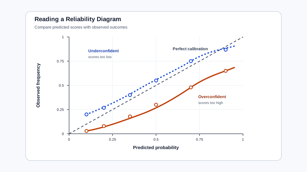
The reliability diagram is the visual diagnostic that reveals whether a model is calibrated. It plots predicted probability on the x-axis against observed frequency on the y-axis. The diagonal line represents perfect calibration: predicted equals observed.

To build one, you bin the predicted scores into groups—say, ten bins from 0 to 1. For each bin, you compute the average predicted probability and the actual positive rate. Then you plot one point per bin.

A perfectly calibrated model sits on the diagonal. Real models deviate in recognizable patterns.

Overconfident models sit below the diagonal at high scores. They predict 0.9 but deliver 0.7, so the curve droops downward. Underconfident models sit above it—they predict 0.6 but deliver 0.8, so the curve rises.

Tree ensembles produce a characteristic sigmoid shape. Because their probabilities cluster near 0 and 1, the curve bows away from the diagonal in the middle: too few predictions land in the moderate range, and the extremes overstate confidence.

The reliability diagram does more than tell you whether calibration is broken. It shows you where the error lives. A model might be well calibrated for low-risk cases but badly overconfident exactly in the high-score range where your decisions matter most.

Measuring How Far Off the Probabilities Are

A diagram gives you the shape of the problem. Numbers let you compare models and track improvement. But each number answers a different question, and picking the wrong one can send you chasing the wrong fix.

The Brier score is the mean squared difference between predicted probabilities and actual outcomes. Lower is better. It evaluates the overall quality of your probabilistic predictions, which means it reflects more than calibration alone. It also rewards sharpness—the useful tendency to produce informative spread rather than predicting the same middle probability for everyone. A model that predicts 0.5 for everything is perfectly calibrated but useless; the Brier score penalizes that lack of sharpness.

Expected Calibration Error (ECE) measures the average gap between predicted and observed frequency across bins. It is intuitive and easy to compute, but it has a weakness: it hides where the error occurs. Two models can have identical ECE while one is badly miscalibrated exactly in the score range you care about.

Log loss is the objective that probabilistic models optimize directly. That is why logistic regression calibrates well by default—it was trained to minimize exactly the error that calibration measures. But log loss also rewards sharpness, so it is not a pure calibration metric either.

Tool	What it shows	What it hides
Reliability diagram	Where predicted and observed frequencies diverge across the score range	No single summary number for model comparison
ECE	One average gap across bins	Which bins contain the error
Brier score	Overall quality of probabilistic predictions	Whether a bad score comes from calibration, weak sharpness, or both

My rule: use a number to compare models, but always look at the reliability diagram to understand what the number is hiding. No single metric tells the whole story.

When Calibration Matters—and When It Does Not

Calibration is not always worth the effort. Before you invest in fixing it, ask one question: do you consume the number or just the order?

Calibration matters when the probability value drives an action. You set a fixed threshold and expect the observed precision to match the predicted value. You allocate budget proportionally to risk scores. You price a product based on predicted default rates. In these cases, a miscalibrated model converts directly into misallocated resources.

Calibration matters less when only the order matters. Ranking candidates for a shortlist, ordering search results, or prioritizing alerts where you pick the top N—these tasks consume the sequence, not the absolute values. A model with perfect ranking and terrible calibration still produces the correct shortlist.

Here is the counterintuitive part: a well-calibrated but mediocre model can be operationally useful, while a great-ranking but miscalibrated model can mislead resource decisions. If you need to know that 80% of the cases you flag will actually be positive, a model with modest AUC but honest probabilities serves you better than a ranking champion that overstates its confidence.

One clarification keeps this example honest: calibration describes behavior across score groups, not a guarantee for every threshold you pick. A well-calibrated model tells you that cases receiving roughly 0.8 are positive about 80% of the time. It does not promise that a decision rule built on that score will hit 80% precision on your actual selected population. Threshold performance still needs to be measured against ground-truth labels for the population, time period, and decision rule you deploy.

Tip: When you need to choose a threshold, do not assume your model's probabilities are trustworthy enough to set it directly. Validate the threshold against ground-truth labels. Calibration fixes the probabilities; it does not remove the need for validation.

Common Mistakes When Treating Probabilities as Truth

The traps that follow from assuming a model's score is a trustworthy probability are predictable. I have watched teams step into each of them.

Reading 0.9 as "almost certainly positive" when the model is overconfident and the true rate is closer to 0.7. The number feels precise, so it earns trust it has not earned.

Setting a fixed threshold from uncalibrated probabilities and expecting observed precision to match the predicted value. The threshold was chosen from numbers that were wrong from the start.

Calibrating on the same data used to train the model. This leaks information and overstates calibration quality. You need a held-out set for calibration, just as you need one for evaluation.

Assuming calibration transfers to a new population. A model calibrated on one distribution can drift on another. If your deployment population differs from your training population—different season, different customer segment, different market—recheck the reliability diagram.

Common mistake: Calibration is not a permanent property you earn once. It is a relationship between a model and a population. Change the population, and the relationship changes.

The Decision Rule

Before you trust any probability, ask whether you consume the number or just the order. If you consume the number, check the reliability diagram and measure the gap. If the curve bows away from the diagonal in the score range where your decisions live, your probabilities need work.

The good news is that calibration is fixable. Scikit-learn's CalibratedClassifierCV exists precisely for this purpose, and the two main approaches handle different failure shapes. Use a sigmoid mapping when you have limited calibration data or the reliability pattern is a smooth monotonic curve. Consider isotonic regression when you have enough held-out data and the pattern is clearly non-sigmoidal—but remember that its flexibility demands more data to fit safely.

That is the natural next step: learning how to actually calibrate your models, and choosing the method that matches the bias you see in your reliability diagram.

References

Research updated Sep 8, 2026