How Regression Trees Choose Splits: Derive Squared-Error Reduction

A classification tree asks which split makes the labels purest. A regression tree has no labels to purify — only numbers that scatter. So what is it actually minimizing?

If you have already worked through how classification trees score splits with Gini impurity or entropy, you know the shape of the answer: score every candidate split, then keep the one that improves the node the most. The regression version keeps that shape but swaps the score. Instead of counting mislabeled points, it measures how far each target value sits from the node's prediction, squares that distance, and adds it up. The split that shrinks that total the most wins.

That is the whole idea. The rest of this article is the arithmetic that makes it precise, plus a worked example you can check by hand.

Why Regression Trees Need a Different Split Score

A classification node predicts a class. Purity means "most of the rows in this node share a label," and Gini or entropy gives that a number.

A regression node predicts a single number — the mean of the target values that land in it. There is no label to purify. The closest analogue is spread: how tightly do the target values cluster around that mean? A node where every target is close to the node mean is a good node. A node where targets are scattered far from the mean is a bad one.

That reframing is why the regression criterion is often called variance reduction. Minimizing the spread around the mean is the same as minimizing the node's variance, and scikit-learn's default squared_error criterion is described exactly that way: it minimizes L2 loss using the mean of each terminal node.

Three assumptions are worth stating up front, because they bound everything that follows:

• Targets are numeric, not categorical.
• Splits are binary and axis-aligned: one feature, one threshold, two children.
• We are scoring one node at a time. The tree never looks ahead to how its grandchildren will turn out.

Notation: Node Predictions and Sum of Squares

Before any derivation, pin down the symbols. Most hand-calculation errors come from mixing up two of them.

Take a node containing $n$ target values, $y_1, y_2, \dots, y_n$. The node's prediction is the mean:

$\bar{y} = \frac{1}{n}\sum_{i=1}^{n} y_i$

The node's sum of squared errors is the total squared distance from each value to that mean:

$\text{SSE} = \sum_{i=1}^{n}(y_i - \bar{y})^2$

The mean squared error is just SSE divided by $n$:

$\text{MSE} = \frac{1}{n}\sum_{i=1}^{n}(y_i - \bar{y})^2$

Here is the distinction that matters: the split score uses sums, not means. If you compare one candidate using SSE and another using MSE, you are comparing two different quantities and the winner is meaningless. Pick one, use it everywhere, and say which one you used.

Note: Minimizing SSE at a node is the same as minimizing that node's variance. Variance is SSE divided by $n$, and dividing by a fixed $n$ does not change which split wins. This is why the criterion shows up under two names — "squared error" and "variance reduction" — and they are the same thing.

Deriving the Error Reduction for One Split

Now the actual derivation. It is short, and every step is arithmetic.

A candidate split picks one feature and one threshold. Every row goes left if its feature value is at or below the threshold, and right otherwise. Each child gets its own rows, its own mean, and its own SSE.

Let the left child hold $n_L$ rows with mean $\bar{y}_L$, and the right child hold $n_R$ rows with mean $\bar{y}_R$. Their errors are:

$\text{SSE}_L = \sum_{i \in L}(y_i - \bar{y}_L)^2, \qquad \text{SSE}_R = \sum_{i \in R}(y_i - \bar{y}_R)^2$

The combined error of the children is simply their sum:

$\text{SSE}_{\text{children}} = \text{SSE}_L + \text{SSE}_R$

The reduction from splitting the parent is the parent's error minus the children's combined error:

$\Delta = \text{SSE}_{\text{parent}} - \left(\text{SSE}_L + \text{SSE}_R\right)$

The tree computes $\Delta$ for every candidate threshold on every feature, then keeps the split with the largest $\Delta$. That is the greedy step: best local improvement, no lookahead.

Why the child sizes matter

Notice what is not in that formula: any explicit weighting by $n_L$ or $n_R$. In the classification case, you weight each child's impurity by $n_{\text{child}}/n$ before subtracting. Here the weighting is already baked in, because SSE is a sum over rows. A child with more rows contributes more terms, so it carries more weight automatically.

That has a consequence worth internalizing. Suppose a split isolates a single extreme point into the left child. That child's SSE is zero — one point, and its mean is itself. Clean, right? But the right child still holds almost every row, and its SSE barely moved from the parent's. The total $\text{SSE}_L + \text{SSE}_R$ is nearly unchanged, so $\Delta$ is tiny. A split that looks surgically clean on one side can be almost worthless overall.

This is the trap. The child that looks pure is not the one that decides the winner. The total does.

Worked Example: Two Candidate Partitions by Hand

Let us run the numbers. Nine students, one feature (hours studied), one target (exam score). Keep it small enough to total by hand.

Hours	Score
1	52
2	55
3	58
4	62
5	70
6	72
7	88
8	92
9	95

Parent node

Sum the scores: $52 + 55 + 58 + 62 + 70 + 72 + 88 + 92 + 95 = 644$.

Parent mean: $\bar{y} = 644 / 9 \approx 71.56$.

Now the squared deviations:

$y_i$	$y_i - \bar{y}$	$(y_i - \bar{y})^2$
52	−19.56	382.5
55	−16.56	274.2
58	−13.56	183.8
62	−9.56	91.4
70	−1.56	2.4
72	0.44	0.2
88	16.44	270.3
92	20.44	417.8
95	23.44	549.4

$\text{SSE}_{\text{parent}} \approx 382.5 + 274.2 + 183.8 + 91.4 + 2.4 + 0.2 + 270.3 + 417.8 + 549.4 = 2172.0$

Candidate A: split at hours ≤ 5

Left child (hours 1–5): scores 52, 55, 58, 62, 70. Mean $= 297/5 = 59.4$.

Deviations: −7.4, −4.4, −1.4, 2.6, 10.6. Squares: 54.8, 19.4, 2.0, 6.8, 112.4.

$\text{SSE}_L = 195.4$

Right child (hours 6–9): scores 72, 88, 92, 95. Mean $= 347/4 = 86.75$.

Deviations: −14.75, 1.25, 5.25, 8.25. Squares: 217.6, 1.6, 27.6, 68.1.

$\text{SSE}_R = 314.9$

$\text{SSE}_{\text{children}} = 195.4 + 314.9 = 510.3$

$\Delta_A = 2172.0 - 510.3 = 1661.7$

Candidate B: split at hours ≤ 8

Left child (hours 1–8): scores 52, 55, 58, 62, 70, 72, 88, 92. Mean $= 549/8 = 68.625$.

Deviations: −16.625, −13.625, −10.625, −6.625, 1.375, 3.375, 19.375, 23.375. Squares: 276.4, 185.6, 112.9, 43.9, 1.9, 11.4, 375.4, 546.4.

$\text{SSE}_L = 1553.9$

Right child (hour 9): score 95. One point, so its mean is 95 and its SSE is 0.

$\text{SSE}_R = 0$

$\text{SSE}_{\text{children}} = 1553.9 + 0 = 1553.9$

$\Delta_B = 2172.0 - 1553.9 = 618.1$

Side by side

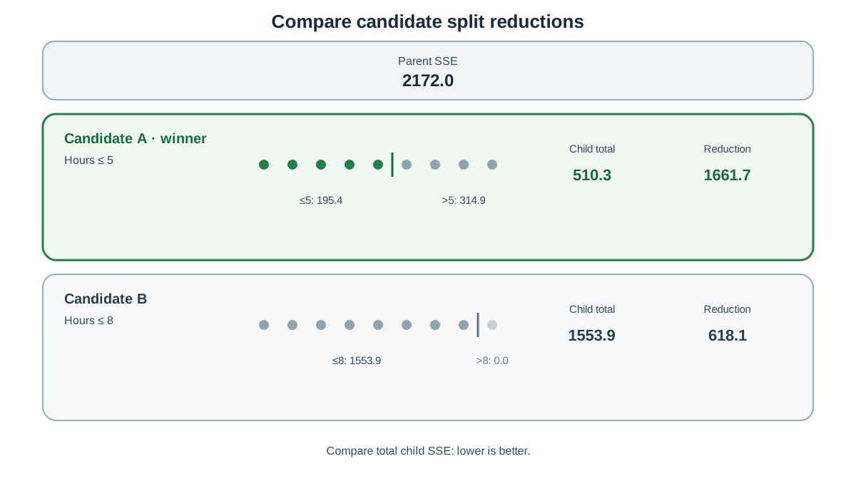
Candidate	Left SSE	Right SSE	Total child SSE	Reduction
A: hours ≤ 5	195.4	314.9	510.3	1661.7
B: hours ≤ 8	1553.9	0.0	1553.9	618.1

Candidate B has a perfectly pure child — zero error on the right. Candidate A has no pure child at all. And Candidate A wins by a wide margin, because its total child error is far lower. This is the trap from the previous section, made concrete: a zero-error child is not the same as a good split.

Confirming with scikit-learn

You can verify the arithmetic with a depth-1 tree. The code is confirmation, not the lesson:

import numpy as np
from sklearn.tree import DecisionTreeRegressor

X = np.array([[1],[2],[3],[4],[5],[6],[7],[8],[9]])
y = np.array([52, 55, 58, 62, 70, 72, 88, 92, 95])

tree = DecisionTreeRegressor(max_depth=1, criterion="squared_error")
tree.fit(X, y)

print(tree.tree_.threshold[0])   # the chosen split threshold
print(tree.tree_.impurity[0])    # parent MSE

The threshold the tree reports should sit between hours 5 and 6, matching Candidate A. The parent impurity it prints is the parent MSE, which is $\text{SSE}_{\text{parent}} / 9 \approx 241.3$ — the same number you computed, divided by $n$.

Reading the Result Correctly

A larger reduction means one thing: a better local fit to the training rows at this node. Nothing more. It is worth being explicit about what that number does not claim.

• It is not evidence of generalization. The same greedy score will happily chase noise. If a handful of rows happen to share a feature value and a target value, the split that isolates them looks great on paper and predicts nothing useful on new data. This is why depth limits, minimum leaf sizes, and pruning exist.
• It is not causal structure. The split reflects a correlation in the training sample. Hours studied and exam score move together here; the tree does not know why, and neither does the reduction.
• It is not a global optimum. Greedy local choices can produce a tree that a different split order would have beaten. The tree takes the best split now and never revisits that decision.

In practice, this criterion interacts with several knobs. min_samples_split and min_samples_leaf stop the tree from making splits that reduce error on too few rows. max_depth caps how many times the greedy step can run. And when squared error is the wrong loss — say, when your targets have heavy outliers — scikit-learn also offers absolute_error (which predicts the median and minimizes L1 loss) and poisson (for count-like targets). Squared error is the default, not the only option.

Common mistake: Treating a large reduction as a measure of model quality. It is a measure of fit to the rows currently in the node. Those are different claims, and confusing them is how people end up with a tree that scores perfectly on training data and poorly everywhere else.

Common Mistakes When Computing Split Scores

These are the errors I see most often when people work through this by hand. Each one silently changes the answer.

• Averaging the child means instead of summing the child SSEs. The score is $\text{SSE}_L + \text{SSE}_R$, not $(\bar{y}_L + \bar{y}_R)/2$. Means describe the children; sums score the split.
• Reusing the parent mean for a child. After the split, each child gets its own mean. Recomputing it is not optional — it is the step that makes the child's SSE small.
• Comparing MSE for one candidate against SSE for another. Pick one unit and stay in it. Mixing them makes the comparison meaningless.
• Assuming the split with the lowest error on one side is best. Candidate B above has a zero-error child and loses. Always total both sides.
• Treating the reduction as model quality. It measures fit to the current training rows, not performance on data the tree has never seen.

Where to Go Next

You now have a reusable check. Take any small numeric dataset, compute the parent SSE, compute the child SSEs for two candidate thresholds, and pick the larger reduction. Then say out loud why that winner is only a local training improvement — because that sentence is the one that keeps you honest when the numbers look impressive.

The concrete next step: fit a depth-1 DecisionTreeRegressor on the same nine rows and confirm the threshold matches your hand calculation. Then raise max_depth and watch what happens. Training error will keep falling as the tree carves the data into smaller and smaller pieces. Held-out error will not follow it down forever. That gap — between a greedy score that always improves and a model that eventually stops generalizing — is exactly the problem that pruning and ensemble methods are built to manage, and it is where this series goes next.