How Decision Trees Score Classification Splits: Gini, Entropy, and Gain

You fit a tree, print it, and there it is: the root splits on worst radius, not mean texture. The library made a choice. You can't say why.

That gap matters. "The tree finds the best split" is not a mental model — it's a placeholder for one. The actual mechanism is a scoring loop: every candidate split is graded by how much class uncertainty it removes, weighted by how many samples land on each side. Learn to run that loop by hand and the library's choice stops being magic.

If you already read a tree as a sequence of partitions, you have the prerequisite. Here we stop asking what the tree looks like and start asking why each cut was chosen.

What a Split Score Actually Measures

A node's impurity is one number describing how mixed its class labels are. A node with 90% one class is nearly pure; a 50/50 node is maximally confused.

A split is scored by comparing the parent's impurity to the size-weighted average of the children's impurity. Whatever impurity disappears in that comparison is the gain. Bigger gain, cleaner separation.

Two impurity families dominate classification trees: Gini and entropy. They answer the same question with different curves, and most of the time they agree on which split wins.

Notation and the Two Impurity Functions

Before any formula, fix the symbols. For a node containing samples from $k$ classes, let $p_j$ be the fraction of samples in that node belonging to class $j$. The fractions sum to 1: $\sum_j p_j = 1$.

That vector of class probabilities is the entire input to both impurity functions.

Gini impurity

$G = 1 - \sum_{j} p_j^2$

Derive it from its plain-language meaning. Pick a random sample from the node, then assign it a random label drawn from the node's own class distribution. What's the probability you mislabel it?

The probability you draw class $j$ is $p_j$. The probability you assign class $j$ is also $p_j$. So the probability of a correct assignment is $\sum_j p_j^2$, and the misclassification probability is $1 - \sum_j p_j^2$. That is Gini impurity.

For a binary problem, write $p$ for the fraction of the positive class:

$G(p) = 1 - p^2 - (1-p)^2 = 2p(1-p)$

At $p = 0$ or $p = 1$ (pure node), $G = 0$. At $p = 0.5$ (balanced), $G = 0.5$. Gini peaks at the balanced node.

Entropy

$H = -\sum_{j} p_j \log_2 p_j$

Entropy measures expected surprise. A pure node surprises you never — every sample has the same label — so entropy is 0. A balanced binary node is maximally uncertain, and with the base-2 convention the unit is a bit: one yes/no question's worth of uncertainty.

For the binary case:

$H(p) = -p\log_2 p - (1-p)\log_2(1-p)$

At $p = 0$ or $p = 1$, $H = 0$. At $p = 0.5$, $H = 1.0$. Entropy peaks at the balanced node too — just on a different scale.

Both functions are concave and symmetric about $p = 0.5$. That shared shape is why they usually rank splits the same way. The scales differ: Gini lives in $[0, 0.5]$ for binary problems, entropy in $[0, 1]$.

Note: These formulas describe the empirical label distribution in the node — the fractions you actually counted. They say nothing about the true data-generating distribution. That distinction becomes important when you start trusting split scores as evidence about the world.

Weighted Impurity Decrease, Step by Step

Now the scoring rule. For a candidate split that sends a fraction $w_L$ of the parent's samples left and $w_R$ right:

$\Delta = I(\text{parent}) - \bigl[w_L \, I(\text{left}) + w_R \, I(\text{right})\bigr]$

Read each term:

• $I(\text{parent})$ is the impurity before the split.
• $I(\text{left})$ and $I(\text{right})$ are the children's impurities.
• $w_L$ and $w_R$ are the fractions of the parent's samples reaching each child, with $w_L + w_R = 1$.

The weights are the whole point. Without them, a split that isolates one sample into a pure leaf would score perfectly — impurity 0 on one side, and who cares about the other. Weighting by child size means a tiny pure child can't dominate the score. The gain has to come from cleaning up a meaningful share of the data.

scikit-learn writes the same quantity in raw counts:

$\frac{N_t}{N}\left(I - \frac{N_{tR}}{N_t} I_R - \frac{N_{tL}}{N_t} I_L\right)$

where $N_t$ is the number of samples at the current node, $N_{tL}$ and $N_{tR}$ are the counts in the left and right children, and $N$ is the total. When you pass sample_weight, all four counts are weighted sums.

That same expression powers the min_impurity_decrease parameter: a split is only accepted if its decrease clears your threshold. Set it to zero and the tree splits whenever any gain exists — which is exactly how you grow a tree that memorizes noise.

Common mistake: Treating the gain as a global optimization. The tree maximizes gain at this node only, with no lookahead. A split that looks mediocre now might have enabled a brilliant split two levels down. Greedy search never finds out.

Worked Example: Scoring Two Candidate Splits

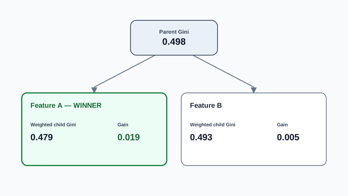
Here is a small binary-class table. Fifteen rows, one label column, two candidate features.

Parent node. Count the labels: eight 0s, seven 1s. So $p_0 = 8/15 \approx 0.533$ and $p_1 = 7/15 \approx 0.467$.

Gini: $1 - (0.533^2 + 0.467^2) = 1 - (0.284 + 0.218) = 0.498$.

Entropy: $-0.533\log_2 0.533 - 0.467\log_2 0.467 \approx 0.533(0.908) + 0.467(1.099) \approx 0.997$.

Candidate 1 — split on Feature A. Left child (A = low): rows 1–8, labels 0,0,1,0,1,1,1,1 → three 0s, five 1s. Right child (A = high): rows 9–15, labels 0,0,0,0,1,1,1 → four 0s, three 1s.

Left Gini: $1 - (0.375^2 + 0.625^2) = 1 - (0.141 + 0.391) = 0.468$.

Right Gini: $1 - (0.571^2 + 0.429^2) = 1 - (0.326 + 0.184) = 0.490$.

Weighted child sum: $(8/15)(0.468) + (7/15)(0.490) = 0.250 + 0.229 = 0.479$.

Gain: $0.498 - 0.479 = 0.019$.

Candidate 2 — split on Feature B. Left child (B = small): rows 1,2,3,9,10 → three 0s, two 1s. Right child (B = medium or large): rows 4–8 and 11–15 → five 0s, five 1s.

Left Gini: $1 - (0.6^2 + 0.4^2) = 1 - (0.36 + 0.16) = 0.48$.

Right Gini: $1 - (0.5^2 + 0.5^2) = 0.5$.

Weighted child sum: $(5/15)(0.48) + (10/15)(0.5) = 0.16 + 0.333 = 0.493$.

Gain: $0.498 - 0.493 = 0.005$.

Feature A wins under Gini. Now repeat with entropy.

Candidate 1, entropy. Left child (3/8, 5/8): $H = -0.375\log_2 0.375 - 0.625\log_2 0.625 \approx 0.375(1.415) + 0.625(0.678) \approx 0.954$. Right child (4/7, 3/7): $H \approx 0.571(0.807) + 0.429(1.222) \approx 0.985$.

Weighted child sum: $(8/15)(0.954) + (7/15)(0.985) = 0.509 + 0.460 = 0.969$.

Gain: $0.997 - 0.969 = 0.028$.

Candidate 2, entropy. Left child (3/5, 2/5): $H \approx 0.6(0.737) + 0.4(1.322) \approx 0.971$. Right child (5/10, 5/10): $H = 1.0$.

Weighted child sum: $(5/15)(0.971) + (10/15)(1.0) = 0.324 + 0.667 = 0.991$.

Gain: $0.997 - 0.991 = 0.006$.

Both criteria pick Feature A. The magnitudes differ — 0.019 versus 0.028 — because the scales differ, not because entropy "found more signal." The ranking is what matters, and here the two criteria agree.

They don't always agree. When two candidates are close in gain, the different curves can flip the winner. That's the tie-breaking regime, and it's where criterion choice actually shows up.

Gini vs Entropy in Practice

Given how similar the two are, how should you choose?

Start with Gini. It's the scikit-learn default, it's cheaper to compute (squares versus logarithms), and on large datasets with many candidate thresholds that cost is real. For most classification problems, the tree you get is effectively the same.

Switch to entropy when you have a reason. If you're comparing against ID3- or C4.5-style behavior, or diagnosing how split selection interacts with feature cardinality, entropy is the criterion those algorithms use.

The cardinality issue is worth understanding. Entropy-based gain is more prone to favoring features with many distinct values or categories. A noisy high-cardinality feature offers more thresholds to try, so it has more chances to score well by luck. Gini's bias in that direction is smaller, which is why CART defaults to it and why C4.5 introduced gain ratio as a normalization.

Tip: If your tree's best splits keep landing on an ID-like column, suspect split bias before you suspect a real signal. Drop the column and refit. If the tree's structure barely changes, the column was noise.

scikit-learn exposes both through the criterion parameter, and log_loss is the same family as entropy for binary classification.

What a Good Split Score Does Not Tell You

A high-gain split is a statement about your training sample. Nothing more.

It doesn't guarantee generalization. Greedy local optimization can build a deep tree that fits noise perfectly. Every split looked good at the time. The tree still fails on held-out data.

It isn't causal. Impurity decrease is not feature importance in any causal sense. A feature can score well because it's correlated with a proxy for the label, or simply because it has many distinct values to try.

It can stall on patterns no single split can separate. The XOR pattern is the classic case: no axis-aligned cut reduces impurity, so a greedy tree stops early even though the classes are perfectly separable by a diagonal boundary.

It can be fooled by cardinality. A noisy high-cardinality feature can outscore a genuinely informative low-cardinality one. Watch for this when a suspicious column keeps winning.

The procedure is reproducible: compute parent impurity, compute weighted child impurity for each candidate, subtract, pick the largest gain. Then treat that number as a local score, not a verdict.

Fit a tree in scikit-learn, print the tree_.impurity array, and check whether the splits the library chose match the ones you scored by hand. When they diverge, you've found either a bug in your arithmetic or a subtlety in the algorithm — and both are worth chasing.