Inspect Random-Forest Out-of-Bag Scores as the Forest Grows

oob_score=True looks like a free validation set. It is not free, and it is not quite a validation set. It is a running estimate computed on the same rows your trees were trained around, from a randomly varying subset of those trees. This tutorial makes that estimate move so you can see where it earns trust and where it quietly drifts.

We will build one controlled experiment: grow a forest tree by tree, record the out-of-bag score at each step, and hold a reserved validation set beside it the whole way. By the end you will have a curve you can read, a script you can rerun on your own data, and a decision rule for when the OOB number is a signal and when it is a story you are telling yourself.

What the OOB Score Actually Measures

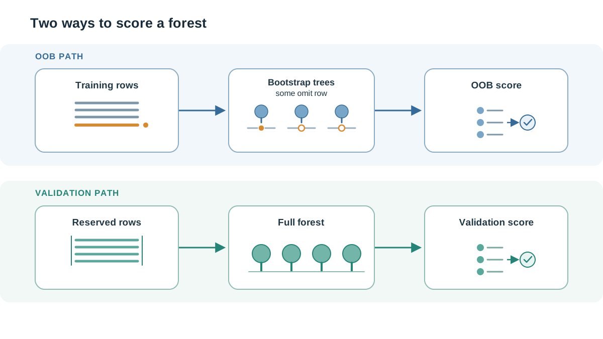
Before any code runs, get the mechanism straight, because the shape of the curve only makes sense if you know what produced it.

Each tree in a random forest is fit on a bootstrap sample: rows drawn from the training set with replacement. Because of that replacement, roughly a third of the training rows never enter any given tree's sample. Those rows are out of bag for that tree.

For a single training row, the OOB prediction uses only the trees that never saw it, then aggregates their votes. The OOB score is the aggregate accuracy over all training rows, where each row is scored by its own private subset of trees.

Two consequences fall out of that definition, and they matter later:

• Different rows are scored by different numbers of trees. That count is random, and for small forests it is small.
• The estimate is not a clean holdout. Every row was available to most of the forest. It was merely withheld from a random fraction of it.

If you have worked through why averaging correlated trees reduces variance, this is the same averaged predictor being measured — just on partially unseen rows instead of fully unseen ones. The averaging still helps. The measurement is just less clean than a reserved split.

Set Up a Controlled Experiment

You need scikit-learn, NumPy, pandas, and matplotlib. No credentials, no external services.

The discipline starts before the first fit: split off a validation set and leave it alone. One honest reference point is enough for this demonstration, and keeping the setup small makes the mechanism easier to see.

import numpy as np
import pandas as pd
from sklearn.datasets import make_classification
from sklearn.ensemble import RandomForestClassifier
from sklearn.metrics import accuracy_score
from sklearn.model_selection import train_test_split

RANDOM_STATE = 0

X, y = make_classification(
    n_samples=4000,
    n_features=20,
    n_informative=8,
    n_redundant=4,
    class_sep=1.0,
    flip_y=0.05,
    random_state=RANDOM_STATE,
)

# Validation set: our honest reference point for the whole sweep.
X_train, X_val, y_train, y_val = train_test_split(
    X, y, test_size=0.25, stratify=y, random_state=RANDOM_STATE
)

print(X_train.shape, X_val.shape)

Expected output:

(3000, 20) (1000, 20)

Everything below happens on X_train and is scored against X_val. If you start tuning against X_val, it stops being a reference point and becomes part of training.

Track OOB as the Forest Grows

The trick is warm_start=True. With it, calling fit again adds trees instead of rebuilding the forest from scratch. Increment n_estimators in a loop, and each step gives you a slightly larger forest and a fresh OOB score.

clf = RandomForestClassifier(
    n_estimators=1,
    warm_start=True,
    oob_score=True,
    random_state=RANDOM_STATE,
    n_jobs=-1,
)

rows = []
for n in range(5, 305, 5):
    clf.set_params(n_estimators=n)
    clf.fit(X_train, y_train)

    oob_error = 1.0 - clf.oob_score_
    val_error = 1.0 - accuracy_score(y_val, clf.predict(X_val))

    rows.append({"n_estimators": n, "oob_error": oob_error, "val_error": val_error})

results = pd.DataFrame(rows)
print(results.head(10).to_string(index=False))

Expected output (your numbers will differ slightly):

 n_estimators  oob_error  val_error
            5     0.1289     0.1213
           10     0.1067     0.1080
           15     0.0960     0.1000
           20     0.0924     0.0947
           25     0.0880     0.0920
           30     0.0858     0.0893
           35     0.0840     0.0880
           40     0.0822     0.0867
           45     0.0804     0.0853
           50     0.0796     0.0840

Plot both error rates on one figure:

import matplotlib.pyplot as plt

plt.plot(results["n_estimators"], results["oob_error"], label="OOB error")
plt.plot(results["n_estimators"], results["val_error"], label="Validation error")
plt.xlabel("n_estimators")
plt.ylabel("Error rate")
plt.legend()
plt.title("OOB vs validation error as the forest grows")
plt.show()

The observable pattern: both curves drop steeply at first, then flatten. The flat region is where adding trees stops buying accuracy. That is the practical answer to "how many trees do I need?" — not a magic number, but the point where the curve stops moving.

Note: The validation curve is noisier because it is computed on 1,000 rows instead of 3,000. Do not read small wiggles as signal. The OOB curve is smoother because it uses every training row, but that smoothness is not the same thing as correctness.

Read the Curve, Not Just the Final Number

The plateau suggests a reasonable n_estimators range, but the plateau location is data-dependent. It is not a universal rule, and it is not a property of random forests in the abstract. It is a property of this configuration on this data.

Two things to notice:

• OOB error is not monotone in forest size. Early points are high-variance because each row is scored by only a handful of trees. A row that happens to be out of bag for three trees gets a three-vote prediction. That is a noisy measurement, and it shows up as a jumpy left side of the curve.
• The plateau is the variance mechanism settling. More trees shrink the averaging variance, which is why the curve flattens. The curve is not proving your model generalizes well. It is proving the forest stopped improving on its own internal estimate.

That distinction matters. A flat OOB curve on a bad configuration is still a flat curve. It tells you the forest has stabilized, not that it is good.

Where OOB and Held-Out Scores Diverge

The two curves above track each other closely. That is the happy case. It is not guaranteed, and the conditions under which they diverge are worth knowing before you trust the number.

Condition	What happens to OOB	What to do
Small training set	Fewer rows are averaged into the estimate, so it is noisy and can be optimistic	Prefer a reserved validation set
Imbalanced classes	Aggregate accuracy can look fine while minority-class recall is poor	Check per-class metrics, not just the score
Many predictors, weak effects	Published work reports OOB overestimating error in these settings	Treat the number as a rough signal, not a verdict
Tuning against OOB	The estimate stops being unbiased	Hold out a set you never tune against

The structural reason behind the first row is worth stating plainly: a row scored by fewer trees resembles a test error from a random fraction of the forest, not from the full forest. As the forest grows, that fraction becomes a larger and more stable sample of the ensemble, and the analogy to a full-forest test error improves. But at small forest sizes, the OOB estimate is measuring something subtly different from what you think it is measuring.

Common mistake: Picking the friendlier number when OOB and validation disagree. A large gap is a reason to investigate, not a reason to choose the estimate you prefer.

Break It on Purpose

The fastest way to internalize the limitations is to make them visible. Shrink the training set dramatically and rerun the sweep.

X_small, _, y_small, _ = train_test_split(
    X_train, y_train, train_size=300, stratify=y_train, random_state=RANDOM_STATE
)

clf_small = RandomForestClassifier(
    n_estimators=1, warm_start=True, oob_score=True,
    random_state=RANDOM_STATE, n_jobs=-1,
)

small_rows = []
for n in range(5, 305, 5):
    clf_small.set_params(n_estimators=n)
    clf_small.fit(X_small, y_small)
    small_rows.append({
        "n_estimators": n,
        "oob_error": 1.0 - clf_small.oob_score_,
        "val_error": 1.0 - accuracy_score(y_val, clf_small.predict(X_val)),
    })

small_results = pd.DataFrame(small_rows)
print(small_results.head(10).to_string(index=False))

What changes: the OOB curve becomes jumpy, and the gap to validation widens. With 300 training rows, the estimate averages over far fewer observations, so each row's noisy prediction carries more weight in the aggregate. The number of OOB trees per row is still governed by the forest size — that part has not changed — but fewer rows now contribute to the average, so the estimate inherits more variance.

What stays stable: the general shape — steep drop, then flatten. The mechanism does not change. Only the reliability of the measurement does.

Record what you would have trusted before running this. That is the debugging habit: change one thing, observe the output, revise the belief.

When to Use OOB and When Not To

Use OOB as a cheap first read on forest size and as a sanity check during development. It is especially useful when data is plentiful and classes are balanced, because then each row gets many OOB trees and the estimate is stable.

Do not use OOB as your only evidence of generalization. Do not use it as a substitute for a reserved set on small or imbalanced data. And do not tune hyperparameters against it — if you do, it stops being an unbiased estimate, and the same leakage logic that applies to any validation set applies here.

My rule: compute both, and treat a large gap as a reason to investigate rather than a reason to pick the friendlier number.

The next experiment is to rerun the sweep with max_features varied. Watch whether the plateau moves. If it does, you have learned something important: the plateau is a property of the configuration, not a fixed law of random forests. That connects this experiment to the broader ensemble-tuning workflow, and it is where the real leverage lives.