Build and Evaluate a Stacking Classifier With Scikit-Learn

A stacking classifier can score beautifully on your test set for a reason that has nothing to do with skill: the meta-model was trained on predictions the base models had already seen. This tutorial builds one the honest way, then checks whether it earned the complexity.

What You Are Actually Building

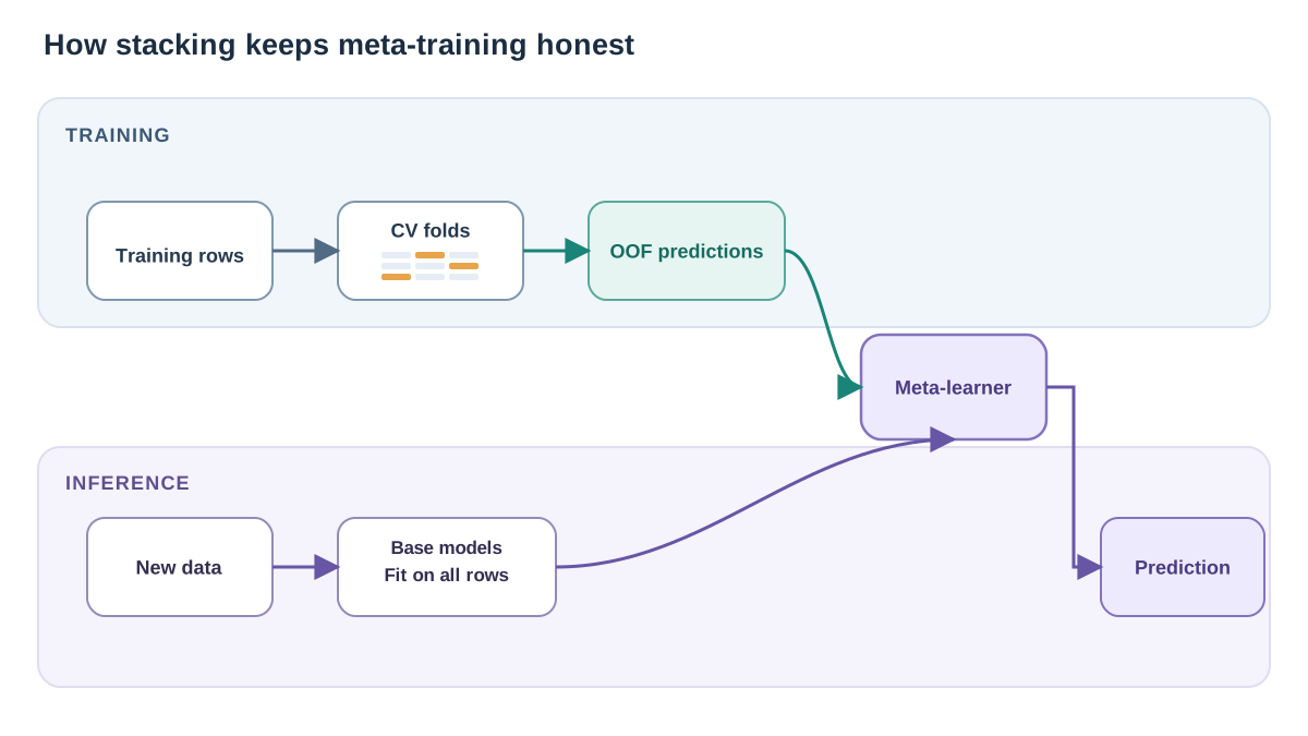
Stacking is a two-level training problem, not voting with extra steps.

At level zero, a set of base estimators each learn to predict the target. At level one, a final estimator — the meta-learner — learns how to combine those predictions into one answer. Voting applies a fixed rule: average the probabilities, or take the majority. Stacking learns the rule.

The mechanism that makes it honest is an asymmetry. In scikit-learn, the base estimators are fitted on the full training set, but the final estimator is trained on cross-validated predictions of those base estimators. Each row of meta-training data is a prediction produced by a model that never saw that row.

Why bother? If the meta-model trained on in-sample base predictions, it would see overconfident, memorized outputs and learn to trust them. It would inherit the base models' overfitting instead of correcting it.

You already know hard and soft voting, and why diverse errors help. The short bridge: stacking can beat voting because it can learn that one base model is reliable on one region of the input space and another is reliable elsewhere. Voting cannot.

The vocabulary you will meet in the API: estimators (the base list), final_estimator, cv (the out-of-fold scheme), stack_method (what each base model emits — probabilities, decision values, or labels), and passthrough (whether the meta-model also sees the original features).

Set Up a Controlled Experiment

Everything that follows depends on fixed conditions. Change the split mid-experiment and every number becomes noise.

You need scikit-learn (any version with StackingClassifier), NumPy, and pandas. No credentials, no external services. We will use a small built-in dataset so the whole run finishes in seconds.

import numpy as np
import pandas as pd
from sklearn.datasets import load_breast_cancer
from sklearn.model_selection import train_test_split

RANDOM_STATE = 42
X, y = load_breast_cancer(return_X_y=True)

X_train, X_test, y_train, y_test = train_test_split(
    X, y, test_size=0.25, stratify=y, random_state=RANDOM_STATE
)

That X_test is now sealed. It gets touched once, at the very end, for the final comparison of the models you have already chosen. Not during model selection, not to "sanity check" a variant, not to pick a fold count.

Success criterion: one table of held-out scores for a baseline, a voting ensemble, and a stacking classifier, all produced by the same evaluation design.

Fit a Baseline Before You Stack Anything

Without a reference point, a stacking score is a number with no meaning. Fit one simple, well-understood classifier first.

from sklearn.linear_model import LogisticRegression
from sklearn.preprocessing import StandardScaler
from sklearn.pipeline import make_pipeline
from sklearn.metrics import accuracy_score

def score_on_test(model, name):
    return {"model": name, "test_accuracy": accuracy_score(y_test, model.predict(X_test))}

baseline = make_pipeline(StandardScaler(), LogisticRegression(max_iter=1000))
baseline.fit(X_train, y_train)
results = [score_on_test(baseline, "baseline (logistic regression)")]
print(results[-1])

The score_on_test helper matters more than it looks. Every model goes through the same code path, so no model gets a friendlier evaluation than another.

Set your expectations honestly here. On small, easy datasets, a single well-regularized model often matches or beats an ensemble. That is a legitimate result, not a failure of the tutorial. The point is to find out, not to confirm a preference.

Build the Stacking Classifier

Now the smallest runnable stack. Each constructor argument maps back to the mechanism.

from sklearn.ensemble import RandomForestClassifier, StackingClassifier
from sklearn.svm import SVC
from sklearn.neighbors import KNeighborsClassifier

base_estimators = [
    ("rf", RandomForestClassifier(n_estimators=200, random_state=RANDOM_STATE)),
    ("svc", make_pipeline(StandardScaler(), SVC(probability=True, random_state=RANDOM_STATE))),
    ("knn", make_pipeline(StandardScaler(), KNeighborsClassifier(n_neighbors=5))),
]

stack = StackingClassifier(
    estimators=base_estimators,
    final_estimator=LogisticRegression(max_iter=1000),
    cv=5,
    stack_method="predict_proba",
    n_jobs=-1,
)
stack.fit(X_train, y_train)
results.append(score_on_test(stack, "stacking"))
print(results[-1])

Four choices deserve a reason.

Base estimator diversity. A random forest, an SVM, and k-nearest neighbors make mistakes in different ways. Three random forests with different seeds would mostly agree, and agreement adds nothing to a meta-model. Diversity is the raw material.

Pipelines around anything that scales. The SVM and k-NN need standardized features. Wrapping them in make_pipeline keeps the scaler inside each cross-validation fold, so the scaler never sees validation rows during fitting. Scaling before the split is one of the most common silent leaks.

A simple final estimator. The meta-model is solving a small weighting problem over a handful of columns. A logistic regression is low-variance and easy to reason about. Reaching for a deep tree here usually just overfits the out-of-fold predictions.

An explicit cv. The default is 5-fold, but writing it down forces you to own the choice. You will change it deliberately in the last section.

Inspect the Out-of-Fold Meta-Features

The stack works, but you should be able to see why. Reconstruct the meta-features yourself with cross_val_predict using the same fold strategy.

from sklearn.model_selection import cross_val_predict

meta_features = np.column_stack([
    cross_val_predict(est, X_train, y_train, cv=5, method="predict_proba")[:, 1]
    for _, est in base_estimators
])

print(meta_features.shape)   # (n_train_samples, n_base_estimators)
print(meta_features[:3])

Each row is one training sample. Each column is one base model's out-of-fold probability that the sample is positive — produced by a model that never trained on that sample. That is the exact matrix the meta-model learns from.

Now look at the optimism gap directly. Compare a base model's out-of-fold predictions against its in-sample predictions:

rf = RandomForestClassifier(n_estimators=200, random_state=RANDOM_STATE)
rf.fit(X_train, y_train)
in_sample = rf.predict_proba(X_train)[:, 1]
oof = cross_val_predict(rf, X_train, y_train, cv=5, method="predict_proba")[:, 1]

print("in-sample accuracy:", accuracy_score(y_train, (in_sample > 0.5).astype(int)))
print("out-of-fold accuracy:", accuracy_score(y_train, (oof > 0.5).astype(int)))

The in-sample number will be higher, sometimes dramatically. The meta-model is trained on the honest, slightly pessimistic version. That is precisely why the final pipeline generalizes: it learned to combine models under conditions that resemble the ones it will face.

One practical detail: at prediction time, the base estimators are refit on the full training set, so training cost is roughly folds × base models, plus one final fit.

Compare Stacking Against Voting and a Single Model

Now the real question. Run the same sealed test set through a soft-voting ensemble of the same base estimators.

from sklearn.ensemble import VotingClassifier

voting = VotingClassifier(estimators=base_estimators, voting="soft", n_jobs=-1)
voting.fit(X_train, y_train)
results.append(score_on_test(voting, "soft voting"))

print(pd.DataFrame(results).to_string(index=False))

That printed table is the result. Read it as three answers to the same question, produced under identical conditions: does the extra machinery buy anything here? Sometimes the baseline wins. Sometimes voting edges out stacking. The table tells you which, and the mechanism tells you why.

Model	How it combines predictions	Rough fit cost
Baseline (logistic regression)	none — single model	lowest
Soft voting	fixed rule: average probabilities	one fit per base model
Stacking	learned weights from out-of-fold predictions	folds × base models + final fit

The mechanism behind the difference: voting applies a rule you chose in advance, stacking learns one from data. Learned weights only pay off when the base models are genuinely diverse and the meta-model has enough rows to learn from.

Common mistake: assuming stacking always wins. With few training samples, the meta-model can overfit the out-of-fold predictions and lose to plain voting. The out-of-fold matrix has only as many rows as you have training samples, and the meta-model is fitting on top of noisy estimates.

A decision rule I would actually use: start with the simple model. Add voting when you want a cheap robustness gain with almost no tuning. Reach for stacking when you have enough data, genuinely different base models, and a reason to believe the right combination is not uniform across the input space.

Failure Modes and Debugging Signals

Symptom	Likely cause	Fix
Suspiciously high test score	Preprocessing fitted outside the pipeline, or the test set used during model selection	Wrap scalers in pipelines; seal the test set until the final comparison
Stacking worse than every base model	Meta-model overfitting on too few out-of-fold rows, or base models too similar	Increase training data, reduce base model count, or drop redundant models
Slow fit, no accuracy gain	Expensive, correlated base estimators	Remove one and re-measure
Confusing estimator count with depth	More base models is not a deeper stack	Multi-layer stacking multiplies cost fast; add layers only with evidence
Comparison table moves between runs	Unseeded base estimators	Set random_state on every stochastic estimator

The first row is the one that bites hardest. A stacking classifier that scores 0.99 on a small dataset is usually not a triumph. It is a leak wearing a nice number.

One Experiment Worth Running Next

Keep the split, the base estimators, and the seeds fixed. Change only the cv strategy used for the meta-features.

Here is the discipline that makes this experiment honest: compare cv settings on a validation split carved out of the training data, not on the sealed test set. If you score every variant against X_test, you are back to selecting on the test set — the exact mistake this tutorial exists to prevent.

from sklearn.model_selection import train_test_split

X_sub, X_val, y_sub, y_val = train_test_split(
    X_train, y_train, test_size=0.25, stratify=y_train, random_state=RANDOM_STATE
)

import time

for k in (3, 10):
    model = StackingClassifier(
        estimators=base_estimators,
        final_estimator=LogisticRegression(max_iter=1000),
        cv=k,
        stack_method="predict_proba",
        n_jobs=-1,
    )
    start = time.perf_counter()
    model.fit(X_sub, y_sub)
    elapsed = time.perf_counter() - start
    print(f"cv={k}: val_acc={accuracy_score(y_val, model.predict(X_val)):.4f} "
          f"fit={elapsed:.2f}s")

Pick the cv setting that looks best on the validation split, refit that configuration on the full X_train, and only then evaluate it once on X_test. That final number is the one you report.

Interpret the result through the mechanism: more folds means less biased out-of-fold predictions, because each base model trains on a larger fraction of the data — but it also means more training runs, and the gain shrinks once folds are large enough.

An optional second variation: add passthrough=True and check whether giving the meta-model the original features helps or just adds noise. On most small tabular problems, it adds noise.

Stacking is a way to learn how to combine models, and it only earns its cost when the base models are diverse and the out-of-fold predictions are honest. The reusable asset here is not the classifier — it is the discipline: one split, one sealed test set, one code path for every score. Carry that into your next ensemble, and tune the meta-model or the fold strategy as the next controlled variable.