
Why a Bootstrap Sample Leaves Observations Out of Bag
A random forest hands you an out-of-bag score, and someone nearby says, "Each tree leaves out about a third of the data." That number feels like a setting.…

Key topics
A random forest hands you an out-of-bag score, and someone nearby says, "Each tree leaves out about a third of the data." That number feels like a setting. It is not. It is a fixed consequence of one sampling rule, and once you derive it, you stop treating OOB as magic and start reading it as a coverage count.
Here is the question worth answering precisely: if I draw a bootstrap sample of size from training rows, what is the probability that one specific row — call it observation — never gets picked at all?
What a Bootstrap Sample Actually Does
Start with the mechanism, because the probability has nothing to attach to until you can picture the draw.
You have training observations. A bootstrap sample draws items with replacement. Each draw picks one of the rows uniformly, so any single row has probability of being chosen on that draw. You repeat this times. The result is a sample of the same size as the original, but it is a multiset: some rows appear twice, some three times, and some never appear.
That last group is the point. The out-of-bag set for one tree is the set of training rows that never appeared in that tree's bootstrap sample. It is not a separate holdout split you carved off. It is a by-product of the resampling itself.
Bagging trains each base learner on its own resample and aggregates the predictions. The OOB set falls out of that process for free. So the real question is not "how many rows are left out" — that varies per sample — but "what is the probability that this specific row is left out." That is a marginal probability, and it is stable.
Knowledge check
Check your understanding
Answer this question before you continue.
Deriving the Omission Probability
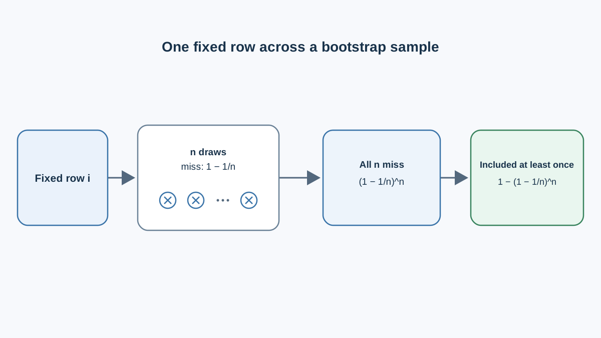
Let's build it one draw at a time. Define as the number of training observations, and fix your attention on a single observation .
Step 1: one draw. On a single draw, the probability that is not selected is the complement of being selected:
Step 2: all draws. The draws are independent and identically distributed. Each draw has the same chance of hitting , and one draw's outcome tells you nothing about the next. For independent events, the probability that all of them miss is the product:
Step 3: the complement. The probability that appears at least once is:
That is the whole derivation. Two lines, one assumption.
Step 4: name the assumption. The result depends on the draws being independent and identically distributed, with each row carrying equal probability . If your resampling scheme weights rows unequally, or draws are somehow dependent, this formula no longer describes your sample. The math is exact only under the standard bootstrap.
Step 5: read the scope. This is a per-observation marginal probability. It does not say "exactly 37% of rows are left out." It says each row, considered on its own, has this chance of being omitted. The actual count of distinct omitted rows in any one sample is a random variable with its own distribution.
Common mistake: Treating as the fraction of rows omitted in a given sample. It is the expected omission probability per row, not a guarantee about any single resample.
Knowledge check
Check your understanding
Answer this question before you continue.
The Large-Sample Limit and Why It Is Roughly 37%
Now push upward and watch what the formula does.
As grows, approaches , which is about . So the omission probability approaches roughly 36.8%, and the inclusion probability approaches about 63.2%.
The convergence is fast enough that the rule of thumb holds at modest sizes. Here are worked numbers:
| Omission | ||
|---|---|---|
| 10 | 0.3487 | ~34.9% |
| 100 | 0.3660 | ~36.6% |
| 1000 | 0.3677 | ~36.8% |
At the gap from is real — about two percentage points — and worth computing rather than assuming. By you are already close.
The limit is a constant, not a function of dataset size. That is why "about a third left out" survives across wildly different datasets. It is baked into the sampling rule, not into your data.
One interpretation worth holding onto: roughly 63% of unique rows appear in a given resample, so the expected number of distinct rows is about . The rest are out of bag.
Note: is a limit, not an exact value. At small , compute the actual probability instead of rounding to 37%.
Knowledge check
Check your understanding
Answer this question before you continue.
From Omission Probability to OOB Coverage
Now scale from one tree to a forest. This is where the per-sample probability turns into something you can observe in a model.
Let be the omission probability for a single tree, and let be the number of trees. For a fixed observation , each tree omits independently with probability . This independence holds because the trees' bootstrap samples are drawn independently under the same sampling rule — that is the standard bagging setup, and it is the condition that makes the count below a clean binomial. The number of trees that can predict is therefore Binomial.
The expected number of OOB trees for a given row is about . With , that is roughly 37 trees. This is why OOB estimates stabilize as the forest grows: more trees means more OOB votes per row, and the average settles down.
The probability that a row is OOB for at least one tree is:
This rises quickly with , but it is never exactly 1 for finite . There is always some chance a row is in-bag for every single tree.
That is the mechanism behind a behavior you may have already hit: scikit-learn's oob_decision_function_ can contain NaN when n_estimators is small, because a data point was never left out during the bootstrap. The math predicted it before the code showed it.
Warning: The derivation describes coverage, not accuracy. It tells you how many trees can vote on a row. It says nothing about whether those votes are any good.
Knowledge check
Check your understanding
Answer this question before you continue.
What the Probability Does Not Promise
The tempting overreach is to conclude that "about 37% left out" means the OOB score is a free, unbiased test score. It is not that simple, and the distinction matters.
Coverage is not independence. For each tree that contributes to a row's OOB prediction, that row was genuinely excluded from training. But the contributing trees are correlated with one another — they were grown on overlapping resamples of the same data — and the OOB estimate is an internal resampling estimate, not a separate external evaluation. The row is held out of the trees that vote on it; the estimate as a whole still lives inside the training data.
OOB error has known weak regimes. It has been reported to behave poorly in settings with small sample sizes, many predictors, weak effects, and balanced classes. Treat it as a useful approximation, not a guarantee.
The arithmetic is configuration-dependent. Change max_samples, and the omission probability changes. Set bootstrap=False, and there is no OOB set at all — scikit-learn only exposes oob_score when bootstrap=True. The ~37% figure assumes the default: draws of size with replacement.
My rule: use OOB as a cheap internal signal while you are developing. Keep a reserved evaluation set for the decisions that actually matter.
Check the Arithmetic Yourself
The derivation earns its keep when it predicts what you observe. Verify it in a few lines.
Compute the limit directly:
import numpy as np

for n in [10, 100, 1000]:
    print(n, (1 - 1/n)**n, 1/np.e)
Then simulate the draw and compare the empirical omission rate to the formula:
import numpy as np

rng = np.random.default_rng(0)
n, trials = 100, 20_000
omitted = sum(0 not in rng.integers(0, n, size=n) for _ in range(trials))
print(omitted / trials, (1 - 1/n)**n)
The two numbers should land close together. That is the point: the formula predicts the output before you run it.
If you want to connect it to a real model, fit a small RandomForestClassifier with oob_score=True and inspect how many trees actually cover each row. Compare the observed counts to the binomial expectation of about . Keep this as verification of the derivation, not a replacement for it.
Where This Leaves You
The ~37% figure is a fixed consequence of sampling times with replacement. It tells you how much OOB evidence exists per row — not how trustworthy that evidence is. Those are two different questions, and conflating them is how people end up trusting an OOB score they should have double-checked.
The next practical step: watch how OOB estimates behave as the forest grows, and compare them against a reserved evaluation set. If the two diverge in a way that surprises you, you have found a regime where coverage was never the whole story.
Knowledge check
Final check
Finish the article by checking the ideas you just learned.
References
Build stronger machine learning foundations
Use structured resources to connect theory, scikit-learn workflows, and evaluation practice.


