
Why Averaging Trees Helps: Derive the Random-Forest Variance Effect
Everyone repeats that a forest reduces variance. Almost nobody writes down the formula that governs the reduction — and that formula contains a term that…

Key topics
Everyone repeats that a forest reduces variance. Almost nobody writes down the formula that governs the reduction — and that formula contains a term that never goes away, no matter how many trees you add.
This is the derivation behind that claim. We will assume every tree has the same marginal variance and that any two trees share one common pairwise correlation, derive the variance of their average, and then work a small numerical example. The result is a model of the mechanism, not a proof about your dataset. Bias is out of scope, and the formula will not predict your held-out error.
What the Variance Claim Actually Says
The quantity we care about is the variance of the average of predictors, not the variance of a single tree. Those are different objects, and conflating them is where most hand-waving starts.
If you have already read why a forest beats a single tree, and how bagging differs from boosting, you have the intuition. This article supplies the algebra. Boosting is sequential error correction; we are only handling the parallel-averaging case here.
Two assumptions do all the work:
- Equal marginal variance. Every tree's prediction has the same variance .
- Common pairwise correlation. Any two distinct trees have the same correlation .
Both are modeling conveniences, not properties of real trees. We will state exactly where they break later. For now, accept them and watch what falls out.
Notation and the Two Assumptions
Fix an input point and fix the training sample. Let
be the predictions of trees at . Each is a random variable because the tree depends on a bootstrap resample of the fixed training data and on the random feature subsets chosen at each split. The training sample itself is held constant; the randomness we are modeling is the tree-construction randomness, not the randomness of drawing a new dataset.
The ensemble prediction is the arithmetic mean:
We assume:
Equal variance is a convenience. Real trees in a forest differ in depth, in which features they split on, and in how much of the data they see, so their variances are not identical. A single correlation parameter is a stronger simplification still: real trees have heterogeneous, data-dependent correlations, and the correlation between two trees depends on where in feature space you evaluate them.
That last point matters. The correlation here is between predictions at a fixed input , not between errors. It is a local quantity. Two trees may agree closely in one region of the input space and disagree sharply in another. The averaging argument is therefore local, not global — it describes what happens at one point, and you would have to integrate over to say anything about overall performance.
Knowledge check
Check your understanding
Answer this question before you continue.
Deriving the Variance of the Average
Start from the definition of variance for a sum, with the constant factor pulled out:
The variance of a sum expands into a double sum over all ordered pairs:
Split that double sum into two parts. When , the covariance is just the variance. When , it is the covariance between two distinct trees.
Now count the terms. There are diagonal entries and off-diagonal entries. Substitute the shared variance and the shared covariance. Since for :
Divide by :
Factor out and you get the closed form:
Read the two terms separately.
The first term, , does not contain . It is the irreducible floor set by the correlation between trees. If every tree made the same mistake, , and the floor equals the variance of a single tree — averaging buys you nothing.
The second term, , is the part averaging can actually remove. It shrinks as .
Now take the limit:
The second term vanishes. The first survives. Averaging can only remove the uncorrelated part of the variance, and it can never remove the correlated part.
Knowledge check
Check your understanding
Answer this question before you continue.
A Small Numerical Example
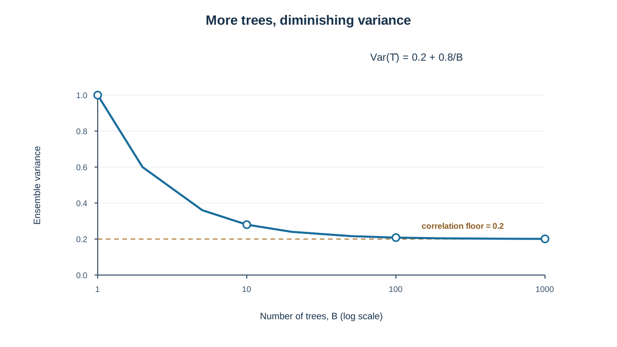
Pick and . Then:
| Trees | Second term | Ensemble variance |
|---|---|---|
| 1 | 0.800 | 1.000 |
| 2 | 0.400 | 0.600 |
| 5 | 0.160 | 0.360 |
| 10 | 0.080 | 0.280 |
| 50 | 0.016 | 0.216 |
| 100 | 0.008 | 0.208 |
| 1000 | 0.0008 | 0.2008 |
The decay is fast at first and then stalls. Going from 1 tree to 10 cuts variance from 1.0 to 0.28 — a 72% reduction. Going from 10 to 1000 cuts it from 0.28 to 0.2008 — another 28%, but you paid a hundredfold in compute. The floor is , and no number of trees will push you below it.
Now hold fixed and vary :
| Correlation | Ensemble variance |
|---|---|
| 0.0 | 0.008 |
| 0.1 | 0.109 |
| 0.2 | 0.208 |
| 0.5 | 0.505 |
| 0.9 | 0.901 |
Changing moves the floor. It does not change the decay rate, which is always . This is the practical reading: past a modest number of trees, more trees buy almost nothing, and only decorrelation lowers the floor.
Knowledge check
Check your understanding
Answer this question before you continue.
From the Formula to Forest Diversity
The formula tells you where to push. If the floor is , then the only lever that lowers it is .
Bootstrap sampling and per-split feature subsampling are both attempts to push down. Bootstrap sampling shows each tree a different resample of the data, so trees disagree about which observations matter. Feature subsampling forces trees to consider different candidate splits, so they disagree about which features matter. Both mechanisms inject disagreement, and disagreement is what lowers .
There is a tradeoff. More aggressive randomization can raise the variance of individual trees — a tree that only sees a random third of the features at each split may be a worse tree than one that sees all of them. It can also change bias. The formula captures only the variance side, and only under the equal-variance assumption. If randomization makes each tree noisier, goes up even as goes down, and the net effect on the ensemble is not obvious from the formula alone.
Keep the causal claim cautious. The formula motivates the design of random forests. It does not prove that any particular randomization scheme helps on a given dataset. That is an empirical question, and it is answered by held-out evaluation, not by algebra.
Knowledge check
Check your understanding
Answer this question before you continue.
Where the Derivation Stops Being True
The formula is a mechanism explanation, and it has clear failure modes.
Real trees are not exchangeable. Their variances differ, and their correlations depend on the input point and on the training data. The equal-variance assumption is a modeling convenience; the common-correlation assumption is a stronger one. When trees have different variances, the algebra still works but the closed form becomes a weighted expression with no single to point at.
The formula says nothing about bias. Randomization can change bias as well as variance. A variance-only account is incomplete, and treating the formula as a full bias-variance decomposition will mislead you. There is active research suggesting that feature randomization can reduce bias relative to plain bagging, not just variance — which the formula above cannot see.
Correlation is not a fixed constant you can read off a fitted forest. It is a modeling assumption, not a measured quantity. You cannot compute from a trained model and plug it in. You can estimate pairwise prediction correlations on held-out data, but that estimate is local to the data you measured it on.
The derivation is conditional on the training sample. It describes the variance of the ensemble's prediction at a fixed input, given the data. It does not describe how the ensemble behaves across resampled datasets. Those are different sources of variability, and the formula only addresses one.
Use the formula to reason about direction and limits, not to predict a number.
What to Take Away
The variance of an average of correlated predictors is:
A floor set by correlation, plus a term that averaging can remove. That is the whole structure.
The practical rule follows directly. Increase ensemble size until the second term is negligible relative to the first, then stop adding trees and attack correlation if you need more. In scikit-learn, that means tuning max_features and the sampling scheme rather than n_estimators.
The honest boundary: the math explains why averaging helps. It does not tell you how much it will help on your data. To find that out, run a controlled experiment. Hold the data split fixed, vary ensemble size and randomization settings, and compare held-out behavior. The formula tells you what to expect in direction. The experiment tells you what actually happened.
Knowledge check
Final check
Finish the article by checking the ideas you just learned.
References
Build stronger machine learning foundations
Use structured resources to connect theory, scikit-learn workflows, and evaluation practice.


