Feature Transformations for Skewed Data: Change the Shape, Not the Meaning

You fit a model to something like house prices or income. Most values bunch on the left, and a long tail stretches to the right. The model behaves strangely: a handful of huge values seem to steer everything. Change one expensive house and your predictions shift. Change a hundred typical ones and nothing moves.

This is not a bug in your code. It is a mismatch between the shape of your data and what your model expects. Feature transformation in machine learning—log transforms, power transforms, and their relatives—exists to fix that mismatch. The trick is understanding what these transformations actually do: they change the shape of your data, not its meaning.

Why a skewed feature can distort your model

Skew is simpler than it sounds. A skewed feature has most values bunched on one side, with a long tail stretching the other way. Right-skewed data—prices, incomes, counts—bunches low and trails high. A few values sit far from the crowd.

That tail becomes a problem when your model relies on distances. Think about what a distance-based algorithm does: it measures how far apart points are. Now imagine a feature where typical values sit between 1 and 10, but a few reach 1,000. The distance between two ordinary points is tiny. The distance between an ordinary point and an extreme one is enormous. The model spends its effort learning to separate the tail from everything else, because that is where the geometric distance lives.

Linear models can struggle for a related reason. The model minimizes a loss—the quantity it tries to make small, like squared error. A few extreme values can contribute so much to that loss that the model contorts itself to predict them well, often at the expense of the bulk of your data.

Two clarifications before we go further.

First, this is not a problem for every algorithm. Tree-based models split on thresholds, so they care only about the order of values, not the gaps between them. A log transform does not change which house is more expensive, so it does not change where a tree draws its splits. If you are using random forests or gradient boosting, you may not need these transformations at all.

Second, this is not the same problem as feature scaling. Scaling divides by a constant—it fixes magnitude differences between features. It does nothing about a long tail within one feature. That requires a nonlinear transformation.

Also, keep one distinction in mind: a long tail is not the same thing as an outlier. A long tail is part of the distribution—many real-world features simply have a few very large values. An outlier is a value that may not belong at all, like a typo or a sensor failure. Transformations can reshape a long tail. They do not automatically repair bad data. If a value is genuinely wrong, fix it first.

What a transformation actually does to your data

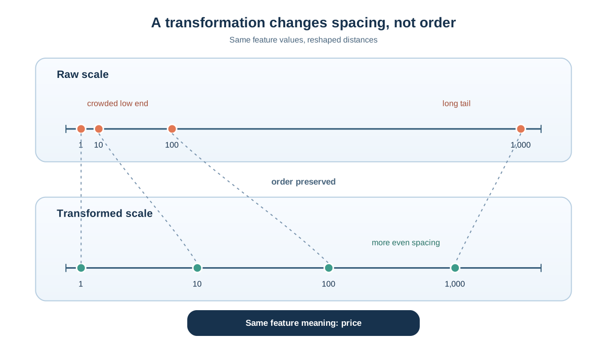
Here is the mental model I want you to keep. Imagine a rubber band with marks drawn along it. The marks are crowded together in one region and stretched far apart in another. A nonlinear transformation is like gripping that rubber band and redistributing the marks—compressing the sparse tail, spreading out the crowded region.

The key word is monotonic. A monotonic transformation preserves the order of values. Bigger stays bigger. If house A costs more than house B before the transform, it costs more after. The ranking is intact. What changes is the spacing between values.

That spacing is what the model sees. After a log transform, the gap between 10 and 100 looks the same as the gap between 100 and 1,000—on the logarithmic scale, both are identical steps. A change in the tail no longer dwarfs a change in the bulk. The model can finally pay attention to differences across the whole range of your data.

This is why I push back on the idea that transformations are cosmetic data cleanup. They are not about making a histogram look prettier. They are about changing the geometry the model learns from—reshaping how far apart points appear without changing what the feature means.

Note: Monotonicity preserves order, but it does not guarantee that every model coefficient keeps its original-unit meaning. After a log transform, a linear model's coefficient describes change in log-space, not in dollars. The feature still means "price," but the model's interpretation of it has changed.

The log transform: the workhorse for right-skewed data

The log transform is the first tool to reach for with right-skewed positive data. Prices, incomes, populations, counts—the log transform is built for these.

Why does it work so well? Because it compresses multiplicative differences into additive ones. A jump from 10 to 100 is a tenfold increase. A jump from 100 to 1,000 is also a tenfold increase. On the raw scale, those jumps look wildly different: 90 units versus 900 units. On the log scale, they are identical steps. The log transform sees the multiplicative structure that the raw scale hides.

There is one practical constraint you will hit immediately: the log of zero or a negative number is undefined. Many real features contain zeros—someone with no income, a count of zero purchases. The standard workaround is log1p, which computes the log of (value + 1). It handles zeros gracefully, though it is not a universal fix for every zero-containing feature. If zero has a special meaning in your data—like "no transaction occurred"—ask whether a transform is even the right tool before applying one.

Power transforms: when log is not enough

The log transform is powerful, but it is not universal. Sometimes the skew is milder, and log over-corrects. Sometimes your data contains zeros or negatives, and log cannot handle them at all.

The square root transform is a gentler option for moderate right skew. It compresses the tail, but less aggressively than log.

When you want the data to choose the transformation, you turn to the power transform family. Box-Cox and Yeo-Johnson are data-driven approaches that search for an optimal power parameter rather than assuming a fixed function like log or square root. They fit a parameter from your data, then apply the corresponding transformation.

The practical difference between them matters. Box-Cox requires strictly positive values. Yeo-Johnson handles zeros and negatives as well. If your feature has negative values, Yeo-Johnson is the option that works out of the box.

Warning: Do not treat these as automatic wins. A data-driven transform can overfit the training distribution, finding a parameter that looks great on your training data but fails on new data. The transform is still a choice you are making, and it needs the same validation discipline as any other modeling decision.

Feature transforms versus target transforms: know which one you are doing

Here is a boundary that beginners often miss. Transforming an input feature and transforming your target variable change different parts of the modeling problem.

A feature transform changes the representation your model learns from. The model still predicts the same thing—house price, income, whatever you set out to predict. Only the input geometry changes.

A target transform changes what the model is optimizing. If you predict the log of house price instead of house price, your model is now minimizing error in log-space. A prediction that is off by 0.1 in log-space corresponds to a different dollar error depending on the price level. To report a meaningful answer, you need to reverse the transform—and the reversal is not always straightforward.

My rule: transform a feature when its shape distorts the model's learning. Transform a target only when you understand that your evaluation and predictions now live in transformed units, and plan accordingly. If your business question is about dollars, make sure your final evaluation reflects dollars.

How to tell if the transformation actually helped

The honest test is not whether the histogram looks more normal. It is whether the model generalizes better on data it has never seen.

This is where beginners often go wrong. They apply a log transform, see a beautiful symmetric histogram, and declare victory. But a prettier distribution can still hurt. The transform may compress the very signal the model needs, or the improvement may be an artifact of the training set.

The right approach is a controlled comparison:

1. Build one model with the raw feature and one with the transformed feature.
2. Evaluate both under the same cross-validation scheme, using the same metric.
3. Compare the mean score across folds—and the spread. A gain that appears in every fold is evidence. A gain that appears in one lucky split is noise.
4. Prefer the simpler representation when the difference is negligible.

Be prepared for the possibility that the transform does not help. If you are using tree-based models, the honest experiment often shows no gain, because trees do not need these transformations. That is a useful result, not a failure. It tells you the raw scale was not the bottleneck.

There is also an operational constraint. A transform applied to training data must be applied identically at prediction time. If your training pipeline applies a log transform and your prediction pipeline forgets it, your model receives data in a different geometry than it learned from. The fix is to make the transform part of a single pipeline that handles both training and prediction.

The decision rule to carry forward

Here is what I want you to remember. When a model seems to chase a few extreme values, suspect a skewed feature distorting the geometry. If the feature is right-skewed and positive, reach for a log transform—the workhorse that compresses multiplicative differences into additive ones. If log is not enough, or your data has zeros and negatives, consider the power transform family. And always let cross-validated generalization—not the shape of the histogram—decide whether the transform earned its place.

The transformation changes the shape of your data. The validation tells you whether that new shape actually helped. The meaning stays with you—it is your job to make sure the model is still learning what you intended.

Once you have a transformed feature that earns its place, the natural next step is learning how to combine these transformations with other preprocessing steps inside a single scikit-learn pipeline—so the same transform applies consistently at training and prediction time, and your validation reflects what your model will actually see in production.

References

Research updated Sep 8, 2026