Run Nested Cross-Validation for Model Selection in Scikit-Learn

You tuned a model, watched the cross-validation score climb, and reported the best number. Then new data arrived and the model performed worse than promised.

Nothing broke. The number was never an estimate of your model's performance. It was an estimate of the best score any candidate could reach on that particular dataset — and those are different quantities.

Nested cross-validation separates the two jobs your single loop was doing at once. Here is the mechanism, a compact scikit-learn implementation, and an honest reading of what comes out.

Why One Cross-Validation Loop Lies to You

If you have already read about cross-validation and hyperparameter tuning, you know the basic setup: split the data into folds, train on some, validate on the rest, average the scores. That machinery is correct. The problem is what you ask it to do afterward.

When you run GridSearchCV, the search evaluates every candidate configuration on the same validation folds and returns the one with the highest score. That maximum is not a neutral measurement. It is the winner of a competition, and winners of competitions look better than average participants. The more candidates you try, and the noisier your folds, the more the winning score drifts above what that configuration will actually deliver on unseen data.

This is not a bug in GridSearchCV. The search is doing exactly what you asked: find the best configuration on this data. The bias enters when you then report that same score as your model's expected performance. You used the data twice — once to choose, once to judge — and the judgment inherited the choice.

Note: Nested cross-validation estimates the performance of the whole procedure — model plus tuning strategy — not of one frozen model. That distinction matters when you interpret the output.

What Nested CV Actually Computes

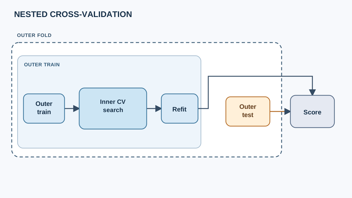
Two loops, two jobs.

The outer loop splits your data into training and test folds. For each outer iteration, the test fold is set aside and never touched during selection. It is the sealed room where you measure what the procedure produces.

The inner loop runs inside each outer training fold. It tunes hyperparameters on its own validation splits and returns a chosen configuration. That configuration is then refit on the full outer training fold and scored once on the sealed outer test fold.

Picture it as nested boxes. The outer fold contains a training portion and a test portion. Inside the training portion, a smaller set of inner folds does the tuning. The outer test block sits outside the inner machinery entirely — visually sealed off, because that is exactly what it is.

The terminology — inner and outer cross-validation — is just a name for this two-level structure. The outer loop estimates. The inner loop selects.

A Minimal Runnable Nested CV Setup

The smallest useful implementation is composition, not a special class. You build a search object with an inner cross-validator, then hand that search object to cross_val_score with an outer cross-validator.

import numpy as np
from sklearn.datasets import load_breast_cancer
from sklearn.model_selection import (
    GridSearchCV, StratifiedKFold, cross_val_score
)
from sklearn.pipeline import Pipeline
from sklearn.preprocessing import StandardScaler
from sklearn.svm import SVC

X, y = load_breast_cancer(return_X_y=True)

pipe = Pipeline([
    ("scale", StandardScaler()),
    ("model", SVC(kernel="rbf")),
])

param_grid = {
    "model__C": [0.1, 1, 10, 100],
    "model__gamma": [0.001, 0.01, 0.1],
}

inner_cv = StratifiedKFold(n_splits=5, shuffle=True, random_state=1)
outer_cv = StratifiedKFold(n_splits=5, shuffle=True, random_state=2)

search = GridSearchCV(
    estimator=pipe,
    param_grid=param_grid,
    cv=inner_cv,
    scoring="accuracy",
    n_jobs=-1,
)

outer_scores = cross_val_score(
    search, X, y, cv=outer_cv, scoring="accuracy", n_jobs=-1
)

print("Per-fold:", np.round(outer_scores, 3))
print(f"Mean: {outer_scores.mean():.3f}  Std: {outer_scores.std():.3f}")

Expected output shape: one score per outer fold, plus a mean and standard deviation. The exact numbers depend on your scikit-learn version and the random seeds, but you should see five values, a mean, and a spread.

Why this works: cross_val_score clones the estimator for each outer fold. The clone is a fresh GridSearchCV that has never seen the outer test data. It runs its inner search on the outer training rows only, picks a configuration, refits, and reports one score. The outer test fold is touched exactly once per iteration.

The validity of the whole procedure rests on one invariant: each inner search sees only its outer training fold. That boundary is enforced by the composition itself — cross_val_score hands the search a training partition, and the search never receives the outer test rows. Separate splitter objects and different random seeds are a convenience for varying fold arrangements, not a correctness condition. Using the same seed for both loops does not leak outer test data; the data boundary is what protects you, not the seed.

One practical choice worth keeping deliberate: use StratifiedKFold for classification. It preserves class proportions across folds, which matters on small or imbalanced datasets.

Reading the Outer Scores Without Fooling Yourself

The mean is the headline, but the per-fold scores are the story.

# Example shape of the output
Per-fold: [0.947 0.965 0.956 0.939 0.974]
Mean: 0.956  Std: 0.013

The spread describes how much the estimate moved depending on which rows landed in which fold. A mean of 0.956 with a standard deviation of 0.013 is a tight cluster. A mean of 0.956 with a standard deviation of 0.08 is a coin flip wearing a decimal point.

Treat that standard deviation as a compact description of variation across these particular outer folds — not a confidence interval, and not a test of independence. The fold scores are dependent by construction, because their training sets overlap. The number tells you how sensitive this run was to the fold arrangement; it does not tell you the precision of your estimate in any formal sense.

Three cautions:

The mean estimates the procedure, not your shipped model. You will eventually refit on all your data with a chosen configuration. That single model has its own variance the nested mean does not capture.

Do not rank models on fine-grained differences when the spread is large. If model A scores 0.956 ± 0.013 and model B scores 0.951 ± 0.014, the gap is smaller than the noise. Pick on other grounds — interpretability, training cost, deployment constraints.

A gap between flat and nested scores is a diagnostic, not a measurement. If your flat GridSearchCV best score was 0.98 and nested CV gives 0.956, that 0.024 difference is consistent with the optimism mechanism — but the two numbers come from different evaluation arrangements, so the gap also reflects fold variation and the different questions each procedure answers. Read it as a signal that selection may be inflating your reported number, not as a quantified bias estimate for this run.

Common mistake: Treating the nested mean as a final model score. Nested CV does not produce a fitted model for deployment. After you have your estimate, refit the chosen configuration on all available data.

Cost, Failure Modes, and Debugging Signals

The compute budget is the reason most people skip nested CV, so let us name it plainly.

Total fits ≈ outer folds × inner folds × candidate configurations, plus one refit per outer fold. With 5 outer folds, 5 inner folds, and 12 candidates, that is 300 fits plus 5 refits. Double the outer folds and you double everything.

That is the real price. Now the failure modes that make the price worthless.

Leakage inside the pipeline. If you scale, impute, or select features before the split, information from the outer test fold bleeds into training. The fix is to put every preprocessing step inside a Pipeline so it is fit inside each fold. The example above does this with StandardScaler — it is not decoration.

Reading the outer test fold to choose between two nested runs. The moment you compare two nested configurations and pick the better one based on outer scores, you have converted your estimate back into a selection signal. The estimate is now biased again.

Forgetting that the inner search must run per outer fold. If you accidentally fit the search once on the full dataset and then evaluate, you have reproduced the flat procedure with extra steps.

Debugging signals worth watching:

• Suspiciously high outer scores — often leakage, or an outer test fold that was accidentally used during tuning.
• Outer scores that match the non-nested number too closely — check that the inner search is actually running inside each outer fold, not once globally.
• Near-zero spread across folds — inspect the context before drawing conclusions. A very homogeneous dataset can produce tight fold scores legitimately; it is not by itself evidence that folds are non-independent.

On parallelism: n_jobs=-1 changes wall-clock time, not the estimate. Use it deliberately, and be aware that nested parallelism (inner and outer both parallel) can oversubscribe your CPU.

When Nested CV Is Worth It — and When It Is Not

Nested CV is not mandatory ceremony. It is a tool with a cost and a specific payoff.

Worth it when: you have many hyperparameter candidates, a small dataset, an unstable model, or a reported number that will drive a real decision or appear in a publication. The selection bias is largest exactly in these conditions.

Not worth it when: your dataset is large, your candidate set is small, or you are doing exploratory work where a rough ranking is enough. A single honest holdout set can answer the question at a fraction of the cost.

There is also research context worth knowing. Wainer and Cawley tested nested versus flat cross-validation across many real binary datasets and concluded that flat cross-validation generally selects an algorithm of similar practical quality to nested CV, provided the learning algorithms have relatively few hyperparameters. The extra cost is not automatically justified.

My rule: if selection is cheap and stable, a single honest holdout is enough. If selection is expensive and noisy — many candidates, small data, high variance — nested CV earns its compute.

One Experiment to Run Next

Run the same model and grid twice: once with a flat GridSearchCV and once with the nested setup above. Put the two numbers side by side.

flat = GridSearchCV(pipe, param_grid, cv=inner_cv, scoring="accuracy", n_jobs=-1)
flat.fit(X, y)
print(f"Flat best CV: {flat.best_score_:.3f}")
print(f"Nested mean:  {outer_scores.mean():.3f}")

Then widen the grid — add more C and gamma values — and watch how the gap changes. More candidates means more chances for the maximum to drift upward. The optimism mechanism stops being theoretical and becomes a number you can see.

If you want to go further, repeat the entire nested procedure with several random seeds and look at how much the outer mean moves. That variation is part of your estimate, not noise to hide.

The same composition pattern extends directly to RandomizedSearchCV and to pipelines with more preprocessing steps. Once you see the inner search as just another estimator being cloned by the outer loop, the structure generalizes.

The habit worth keeping: report per-fold spread, not a single flattering number. A score without its variation is a claim without its error bars.