
Measure the Effects of Label Noise With a Controlled Classifier Experiment
You already know noisy labels hurt models. Knowing it changes nothing. The moment you flip a known fraction of labels yourself, retrain, and watch the…

Key topics
You already know noisy labels hurt models. Knowing it changes nothing. The moment you flip a known fraction of labels yourself, retrain, and watch the score move, the claim stops being a warning and becomes a measurement you own.
This tutorial is that measurement. You will take a clean dataset, corrupt a documented percentage of the training labels, retrain the same classifier at each noise level, and score every run on the same untouched test set. By the end you will have a small table showing how sensitive one model is to one kind of label noise — and a clear sense of what that table does and does not prove.
Why a Controlled Corruption Beats a Vague Warning
The reason to run this experiment instead of reading about it is control. When you corrupt labels on purpose, you know the ground truth. You know exactly which labels you flipped, how many, and in which direction. That lets you separate two things that are usually tangled together in real projects: the model got worse, or the labels got worse.
Here is the mental model for the whole article. Label noise is not a mystery you can only fear. It is a variable you can hold in your hand. You choose the level, you apply it, you measure the result.
Three pieces make the experiment honest:
- A fixed split. You partition the data into train and test once, and reuse that exact partition for every noise level. If the split moves between runs, you cannot tell whether a score changed because of the labels or because of a different test set.
- A documented corruption. You know the fraction of labels you flipped and the rule you used to flip them.
- A clean test set. You never corrupt the test labels. The test set is your measuring stick, and a bent ruler measures nothing.
One boundary up front, because it matters more than the result: this experiment shows the sensitivity of one model on one dataset under one noise type. It is evidence about a direction, not a universal law about robustness. Hold that thought — we will return to it when reading the numbers.
Set Up a Reproducible Experiment
We will use a small, well-understood classification dataset so the clean baseline is trustworthy. The exact dataset matters less than the discipline around it. Pick something small enough to retrain in seconds, because you will retrain it several times.
The setup has three jobs: load the data, fix the split, and create a dedicated random generator for the corruption step. Keeping the split randomness and the corruption randomness separate is the difference between a clean experiment and a confusing one.
import numpy as np
from sklearn.datasets import load_breast_cancer
from sklearn.model_selection import train_test_split
from sklearn.linear_model import LogisticRegression
from sklearn.metrics import accuracy_score

# Load a small, clean, binary classification dataset
data = load_breast_cancer()
X, y = data.data, data.target

# Fix the split ONCE. Reuse these exact arrays for every noise level.
X_train, X_test, y_train_clean, y_test = train_test_split(
    X, y, test_size=0.25, random_state=42, stratify=y
)

# A dedicated generator for corruption, separate from the split seed.
rng = np.random.default_rng(7)

print("Train size:", X_train.shape[0])
print("Test size:", X_test.shape[0])
Two seeds appear here on purpose. random_state=42 fixes the split. default_rng(7) drives the corruption. If you let one generator do both jobs, changing the noise level could silently reshuffle your split, and you would be comparing runs that used different test sets without realizing it.
Now record the baseline. Train on the clean training labels and score on the clean test set.
def fit_and_score(X_train, y_train, X_test, y_test):
    model = LogisticRegression(max_iter=1000)
    model.fit(X_train, y_train)
    preds = model.predict(X_test)
    return accuracy_score(y_test, preds)

baseline = fit_and_score(X_train, y_train_clean, X_test, y_test)
print(f"Baseline accuracy (clean labels): {baseline:.3f}")
That baseline is your reference point. Every later score is read against it. If the baseline itself looks suspiciously low, stop and fix that first — a weak baseline makes the whole sweep unreadable.
Knowledge check
Check your understanding
Answer this question before you continue.
Write the Corruption Function
Now the core mechanic. A corruption function takes labels, a noise fraction, and a random generator, and returns a new set of labels with a chosen proportion flipped to a different class.
def corrupt_labels(y, noise_fraction, rng):
    y_noisy = y.copy()
    n = len(y_noisy)
    n_flip = int(noise_fraction * n)

    # Choose which positions to flip
    flip_indices = rng.choice(n, size=n_flip, replace=False)

    # For binary labels, flipping means moving to the other class
    y_noisy[flip_indices] = 1 - y_noisy[flip_indices]
    return y_noisy
A few decisions are baked into this function, and you should be able to name them:
- Uniform flips. Each selected label moves to the other class regardless of what it was. This is random noise, not systematic noise. A different rule — say, only flipping one class into the other — would produce a different curve.
- Training labels only. The function is applied to
y_train_clean, never toy_test. This separation is the entire point. Corrupt the test set and you have destroyed your ability to measure anything, because your ruler is now wrong in an unknown way. - A documented fraction.
noise_fraction=0.2means roughly 20 percent of training labels change.
Always sanity-check the count. The requested fraction and the actual number of changed labels should match.
y_check = corrupt_labels(y_train_clean, 0.2, rng)
changed = np.sum(y_check != y_train_clean)
print(f"Requested: {int(0.2 * len(y_train_clean))}, Actually changed: {changed}")
Common mistake: Corrupting the test set along with the training set. It feels symmetrical and it is fatal. Your test labels define correctness; if they are wrong, a lower score might mean the model got better at the truth you just erased.
Knowledge check
Check your understanding
Answer this question before you continue.
Run the Sweep Across Noise Levels
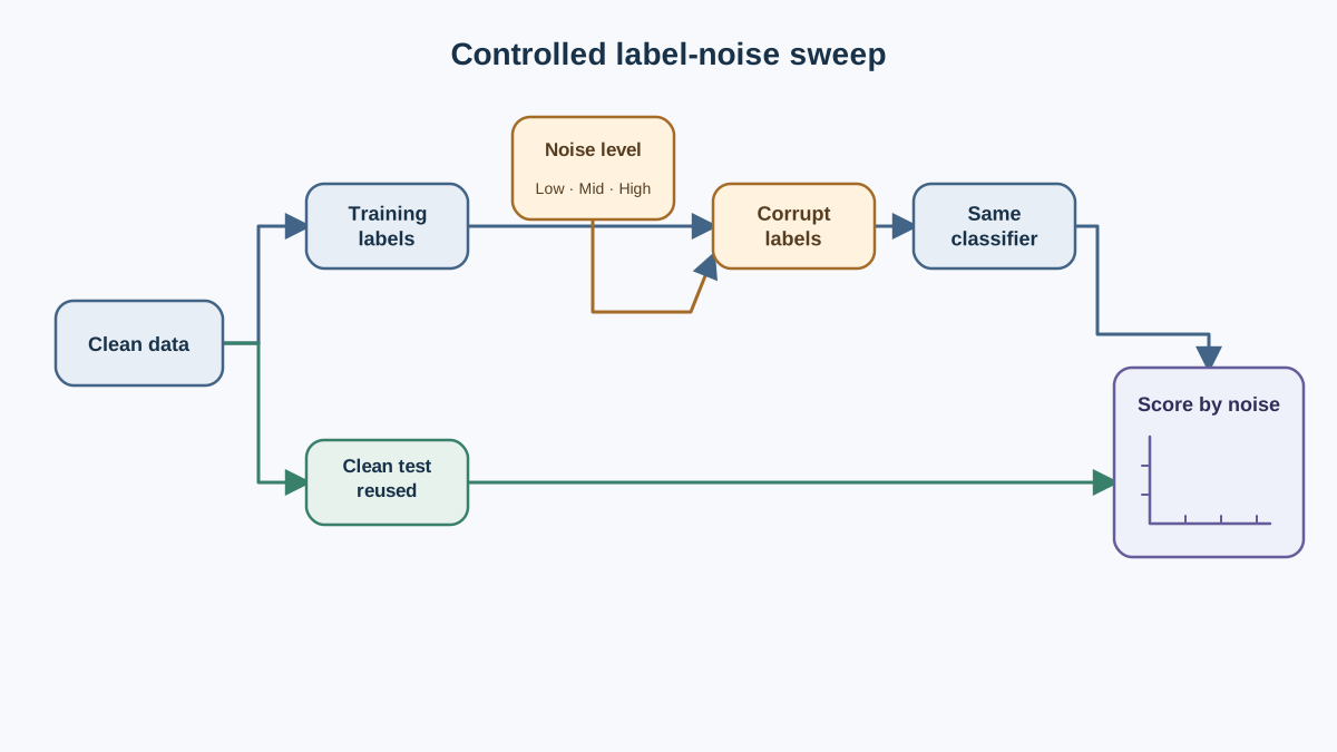
With the pieces in place, the experiment is a loop. For each noise level: corrupt the training labels, retrain the same model with the same hyperparameters, and score on the clean, fixed test set.
noise_levels = [0.0, 0.1, 0.2, 0.3]
results = []

for level in noise_levels:
    y_train_noisy = corrupt_labels(y_train_clean, level, rng)
    score = fit_and_score(X_train, y_train_noisy, X_test, y_test)
    results.append((level, score))
    print(f"Noise {level:.0%} -> test accuracy {score:.3f}")
The output is a table of noise level against test score. Do not expect a perfectly smooth decline. Each level draws a fresh random subset of labels to flip, so the corruption at 20 percent is not a superset of the corruption at 10 percent. Finite-sample variation can make one level score slightly higher than the one below it, and that is not a bug. It is the ordinary noise of a single run.
| Noise level | Test accuracy |
|---|---|
| 0% | baseline |
| 10% | usually below baseline |
| 20% | usually lower still |
| 30% | often the lowest |
Two choices keep this sweep honest. First, the model is not retuned at each noise level. You are measuring sensitivity, not chasing the best possible score under each condition. If you tuned hyperparameters per level, you would be measuring how well you can rescue a model, which is a different question. Second, the same rng carries through the loop, so the corruption at each level is reproducible — but reproducible is not the same as nested. If you want a strictly increasing amount of corruption, sort one random ordering and flip progressively longer prefixes of it. That change makes each level a superset of the previous one and removes the wobble from the comparison.
Knowledge check
Check your understanding
Answer this question before you continue.
Read the Results Without Overclaiming
Look at your table. The scores often fall as noise rises, but a single sweep can wobble, and the direction is the least interesting part anyway. The slope and shape carry the information: does accuracy drop gently, or fall off a cliff between two levels? A gentle slope suggests the model tolerates this noise type; a cliff suggests a threshold past which it stops learning the real pattern.
The mechanism behind the drop is worth stating plainly. The model is fitting a target that is partly wrong. When 20 percent of the training labels point at the wrong class, the model spends part of its capacity learning patterns that do not exist in reality. It is not failing because it is weak. It is succeeding at the wrong task.
Here is where discipline matters. From one sweep you can say: on this dataset, with this model, under uniform random flips, accuracy moved by this much. You cannot say: this model is robust to label noise. That is a universal claim, and you have one data point's worth of evidence.
Several confounders move the curve, and naming them keeps you honest:
- Dataset size. More training data dilutes the effect of a fixed fraction of noise.
- Class balance. If one class is rare, flipping its labels does disproportionate damage.
- Model flexibility. A more flexible model may fit the noise harder and degrade faster — or, in some regimes, average it out.
- Noise type. Uniform flips are the gentlest kind. Systematic or class-conditional noise often hurts more.
Note: A single sweep proves a direction on one setup. Treat it as a hypothesis about sensitivity, not a verdict about the model.
Look Past the Headline Score
Accuracy is one number, and one number hides which mistakes changed. Move to error patterns and the picture sharpens.
To keep the analysis tied to the runs you already scored, store the fitted model and its predictions inside the sweep instead of refitting later. That way the confusion matrices describe the exact runs behind your table.
from sklearn.metrics import confusion_matrix

runs = {}

for level in noise_levels:
    y_train_noisy = corrupt_labels(y_train_clean, level, rng)
    model = LogisticRegression(max_iter=1000).fit(X_train, y_train_noisy)
    preds = model.predict(X_test)
    runs[level] = {
        "score": accuracy_score(y_test, preds),
        "matrix": confusion_matrix(y_test, preds),
    }

print("Low noise:\n", runs[0.1]["matrix"])
print("High noise:\n", runs[0.3]["matrix"])
Now the matrices come from the same corruption draws and the same fitted models as the scores. You are looking for asymmetric damage: noise frequently hurts one class or one direction of error more than the other.
Watch for a stable accuracy that still hides a reshuffled error pattern. If the total number of mistakes barely moves but the kinds of mistakes shift, and those error types carry different real-world costs, your model changed in a way the headline score never reported. This is the same lesson that applies to any single metric: one score rarely describes model quality completely.
The practical payoff is location. Error patterns tell you where the noise is doing its damage, which is exactly what you need before deciding whether to clean labels, reweight samples, or change the model.
Knowledge check
Check your understanding
Answer this question before you continue.
Failure Modes and Debugging Signals
This experiment fails in a handful of predictable ways. Each has a recognizable signal.
- Corrupting the test set by accident. Signal: every score looks terrible, even at 0 percent noise. Fix: confirm the corruption function only ever touches
y_train. - A wobble you mistake for a bug. Signal: one noise level scores slightly higher than the level below it. Fix: this is normal finite-sample variation, not a failure. Repeat each level with different corruption seeds before drawing a conclusion.
- Flips that preserve class balance by accident. Signal: the effect you expected never appears. Fix: check that your flip rule actually changes the class distribution the way you intended.
- A model too simple to learn. Signal: noise appears harmless because the model barely learned anything to begin with. Fix: confirm the clean baseline is meaningfully above chance before trusting the sweep.
- Reading one run as a trend. Signal: a confident conclusion from a single pass. Fix: repeat each noise level with different seeds and look at the variation, not just the mean.
Tip: When a result surprises you, resist the urge to explain it. Reproduce it first. A surprise that survives three seeds is a finding; a surprise that vanishes is a bug.
Extend the Experiment
The sweep you just ran is a template. One meaningful change turns it into a reusable investigation.
Change the noise type. Compare uniform random flips against class-conditional flips, where only one class gets corrupted. The curve often steepens, because you are now teaching the model a biased boundary rather than symmetric confusion.
Change the model. Swap the logistic regression for a more flexible model and rerun the sweep. Does the curve steepen or flatten? The answer tells you something about how that model's capacity interacts with wrong targets.
Repeat each level. Run each noise level several times with different corruption seeds. Now you can separate a real trend from run-to-run variation, which is the difference between a demo and evidence.
Add a cleaning step. Detect likely noisy labels, remove or relabel them, and check whether performance recovers. This connects the experiment to the practical question every real project faces: is it worth cleaning the data?
Keep the fixed split throughout. Every comparison stays honest only as long as the test set never moves.
Where This Leaves You
The habit worth keeping is simple. Whenever you suspect label quality is limiting a model, do not reach for a general claim about robustness. Corrupt the labels on purpose, hold the split fixed, and measure the sensitivity yourself. You will learn more from one honest sweep than from a shelf of warnings.
Start with the next move: rerun this sweep with a second model, or with class-conditional noise instead of uniform flips. Compare the two curves. The gap between them is where your real understanding of label noise begins — and remember that what you observe on one setup is evidence, not a law.
Knowledge check
Final check
Finish the article by checking the ideas you just learned.
References
Build stronger machine learning foundations
Use structured resources to connect theory, scikit-learn workflows, and evaluation practice.


