
Run a Scikit-Learn Error Analysis: Find Slices and Choose a Next Experiment
Your model reports 0.91 accuracy. That number is probably correct, and it is probably useless for deciding what to fix next.

Key topics
Your model reports 0.91 accuracy. That number is probably correct, and it is probably useless for deciding what to fix next.
An aggregate metric answers how often the model is wrong. It says nothing about where or why. Two classifiers can post identical accuracy while failing on completely different rows, and the score cannot tell them apart. Error analysis is how you recover that lost detail: you inspect held-out predictions, group failures into slices, form a hypothesis about the cause, and run one targeted experiment. This article walks through that loop end to end. By the end you will have a slice table, one written hypothesis, and one chosen experiment.
I'm assuming you already know how to pick a metric and have seen the general error-analysis workflow. Here we focus on execution.
Why One Score Is Not a Diagnosis
A summary is where detail goes to die. Accuracy compresses thousands of individual decisions into a single ratio, and in doing so it throws away the structure you need to act on.
Consider a model that predicts whether a support ticket will escalate. It scores 0.91 overall. But suppose it is nearly perfect on tickets from one region and barely better than chance on another. The aggregate number hides that entirely. You would ship the model, and the second region would quietly suffer.
The fix is to treat error analysis as a diagnostic loop, not a report:
- Inspect failures on data the model never saw.
- Form a hypothesis about the mechanism.
- Run one experiment that tests it.
- Re-measure and decide.
The loop matters because a slice you find by exploration is a hypothesis, not a fact. Confirming it requires fresh evaluation, not a second read of the same rows.
Set Up Held-Out Predictions You Can Trust
Everything downstream depends on one artifact: a predictions table built from data the model did not train on. If you inspect in-sample predictions, the model looks better than it is, and you will chase slices that do not exist.
You need Python with scikit-learn, pandas, and NumPy, plus three inputs: a feature matrix X, a target vector y, and an estimator or pipeline. The estimator does not need to be fitted — cross_val_predict fits a fresh clone on each fold internally, so you pass the unfitted object directly.
import numpy as np
import pandas as pd
from sklearn.model_selection import cross_val_predict
from sklearn.ensemble import RandomForestClassifier

clf = RandomForestClassifier(n_estimators=300, random_state=0)

# Out-of-fold predictions: every row is predicted by a model that never saw it.
proba = cross_val_predict(clf, X, y, cv=5, method="predict_proba")[:, 1]
pred = (proba >= 0.5).astype(int)

preds = X.copy()
preds["y_true"] = y.values
preds["y_pred"] = pred
preds["proba"] = proba
The result is one row per example, carrying the true label, the predicted label, the predicted score, and every raw feature you might want to slice on.
Now fix the split-use contract before you look at anything. The out-of-fold predictions are your exploration set: you may slice them, inspect rows, and compare candidate experiments here. Keep a separate final test set untouched. It is your confirmation set, and you spend it once, at the end, on the single experiment you chose. If you explore and confirm on the same rows, the improvement you measure is partly the result of your own search.
Sanity check before moving on: the accuracy of preds should match the metric you already computed. If it does not, your split or your threshold is wrong, and every slice you find afterward will be built on sand.
Build the Error Table Before You Slice
Rates tell you a slice is bad. Rows tell you what the model was looking at when it went wrong. Build the error table first.
preds["is_error"] = (preds["y_pred"] != preds["y_true"]).astype(int)

# For binary problems, separate the two error types.
preds["error_type"] = np.select(
    [
        (preds["y_true"] == 1) & (preds["y_pred"] == 0),  # false negative
        (preds["y_true"] == 0) & (preds["y_pred"] == 1),  # false positive
    ],
    ["false_negative", "false_positive"],
    default="correct",
)
False positives and false negatives usually have different causes. A false negative often means the model lacked a signal that was present; a false positive often means it over-weighted a misleading one. So "most confident mistake" means two different things depending on direction, and a single sort by proba will only show you one of them.
For a false positive, confidence is a high score. For a false negative, confidence is a low score. Inspect both ends:
errors = preds[preds["is_error"] == 1]

# Most confident false positives: high score, wrong positive call.
fp = errors[errors["error_type"] == "false_positive"].sort_values(
    "proba", ascending=False
)

# Most confident false negatives: low score, missed positive.
fn = errors[errors["error_type"] == "false_negative"].sort_values(
    "proba", ascending=True
)

print(fp[["y_true", "y_pred", "proba"]].head())
print(fn[["y_true", "y_pred", "proba"]].head())
These are the rows that betray a broken assumption: the model was most sure and most wrong. Read a handful of them by hand. The pattern you notice in ten rows is often the hypothesis you will test next.
Knowledge check
Check your understanding
Answer this question before you continue.
Slice by Features That Could Plausibly Matter
A slice is a subgroup of rows defined by a feature value or range. The discipline is to slice only on dimensions you can justify before looking at the results. If you slice until something looks bad, you will always find something.
Slice on categorical features directly, bin numeric features into ranges, and try a few combinations. Then compare each slice against the overall error rate — and against the slice size.
overall = preds["is_error"].mean()

def slice_table(df, column):
    g = df.groupby(column)["is_error"].agg(["size", "mean"])
    g.columns = ["n", "error_rate"]
    g["gap_vs_overall"] = g["error_rate"] - overall
    return g.sort_values("gap_vs_overall", ascending=False)

print(f"Overall error rate: {overall:.3f}")
print(slice_table(preds, "region"))
A slice table is the deliverable of this section: slice, n, error rate, and gap versus overall. Read it with suspicion.
| Slice | n | Error rate | Gap vs overall |
|---|---|---|---|
| region = north | 412 | 0.19 | +0.10 |
| region = south | 388 | 0.08 | −0.01 |
| region = east | 4 | 1.00 | +0.91 |
That last row is the trap. A 100% error rate on four rows is noise, not a finding. Small slices, overlapping slices, and slices defined after the fact are the fastest route to a false discovery. Require a slice to be large enough that its gap could not easily be chance before you take it seriously.
Warning: An exploratory slice is a hypothesis, not proof. Confirming it requires a fresh evaluation on data you have not yet inspected.
Knowledge check
Check your understanding
Answer this question before you continue.
Turn the Worst Slice Into a Hypothesis
A hypothesis names a cause and predicts an observable change. "The model is bad on the north region" is not a hypothesis — it is a restatement of the slice. "The model fails in the north because the region feature is missing for those rows, so repairing the feature should close the gap" is a hypothesis you can test.
Before writing it, check the cheap explanations using the error table. Are the confident errors concentrated in one class, one feature range, or one label value? The common causes are worth distinguishing:
- Missing or uninformative features — the signal exists but the model cannot see it.
- Label noise — the target is wrong for some rows in the slice.
- Distribution differences — the slice looks unlike the training data.
- Threshold placement — the errors are near the decision boundary, not deep in the wrong region.
- Model capacity — the pattern is real but the model is too simple to capture it.
Write the hypothesis down in one sentence before touching the model. An unwritten hypothesis mutates to fit whatever result you get, which is how you end up fooling yourself.
Common mistake: Slicing repeatedly until something looks bad. Pre-commit to the slices you will examine, then stop.
Knowledge check
Check your understanding
Answer this question before you continue.
Choose One Targeted Next Experiment
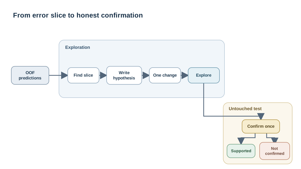
Match the experiment to the hypothesized cause, and change one thing at a time. A bundle of changes teaches you nothing when the score moves.
| Hypothesized cause | Targeted experiment |
|---|---|
| Missing feature | Add or repair the feature |
| Label noise | Inspect and relabel a sample of the slice |
| Distribution difference | Add slice-representative training data |
| Threshold placement | Adjust the decision threshold |
| Model capacity | Increase model complexity |
Define the success criterion before running: which slice should improve, and by how much, without regressing the overall metric.
A short worked example of the loop: you observe a slice gap in the north region. You check the error table and notice the confident errors cluster where a key feature is null. You hypothesize that the missing feature is the cause. You add a repaired version of that feature, refit, and re-measure the slice on the exploration set. If the gap closes there, you have a candidate worth confirming — not a confirmed result. You then run that single change once against the untouched test set. If the gap closes there too, the hypothesis has survived an honest test. If it does not, the hypothesis was wrong, and you have learned something real.
The failure modes here are consistent. Tuning repeatedly on the final test set. Chasing a slice too small to matter. Treating a slice improvement as proof of the underlying cause when it is only consistent with it.
Knowledge check
Check your understanding
Answer this question before you continue.
Keep the Loop Honest
Every exploratory look at held-out data spends some of its value. Track how many times you have looked and on which split. If you keep slicing and re-measuring on the same exploration set, you will slowly overfit to it, and the gap you "fixed" may not exist in production.
Confirm a promising slice on data the exploration did not touch. If it survives, it becomes a real finding worth a data or labeling fix. If it does not, you have learned the aggregate score was telling the truth.
Record the slice definition, the hypothesis, the experiment, and the outcome. The next person needs to reproduce your reasoning, not just your number.
What to Do Next
Here is the decision rule. If the slice gap survives a fresh evaluation on the untouched test set, treat the hypothesis as supported and fix the data or the feature. If it does not survive, do not force the fix — the gap was likely exploration noise, and the aggregate score was telling the truth. Either way, write down what you learned before starting the next loop.
From here, the natural next step is calibration and threshold choice — the score your model produces is not the same as the decision you make with it, and the boundary between them is where a lot of slice-level error actually lives. If you work with regression instead, the same diagnostic instinct shows up as residual analysis: the errors themselves carry the structure the metric flattened.
Knowledge check
Final check
Finish the article by checking the ideas you just learned.
Build stronger machine learning foundations
Use structured resources to connect theory, scikit-learn workflows, and evaluation practice.


