Interpreting Classical ML Models: Rules, Weights, and What They Do Not Prove

"The model says education matters" sounds like a complete explanation. It is not. It is the beginning of a much narrower claim: the model leaned on education to make its predictions. Those two statements feel alike, and confusing them is the most expensive mistake in machine learning explainability.

Interpretation tools answer a specific question: what does the fitted model use to predict, given the data representation and reference distribution you chose? They do not answer a different, bigger question: what causes the outcome in the real world? The first question is about the model you trained. The second requires experiments, domain knowledge, and a level of evidence no fitted model can supply on its own.

This article compares the main ways to interpret classical models—linear coefficients, tree rules, global feature importance, and local explanations—so you can match the tool to the question. Along the way, we will look at where each method misleads, and how to test whether an explanation is stable enough to act on.

What Interpretation Actually Answers

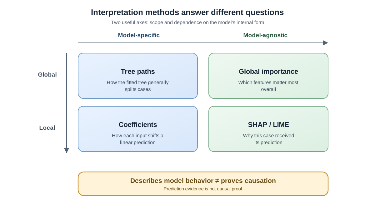
Every interpretation method sits on two axes. The first axis is scope: global methods describe what the model relies on across the whole dataset, while local methods explain a single prediction. The second axis is dependence: model-specific methods read the model's internal structure directly, while model-agnostic methods treat the model as a black box and probe it from the outside.

Here is the concrete contrast that makes the second axis stick: a tree path reads the fitted structure itself, while LIME builds a small neighborhood approximation around one prediction and reads that surrogate instead. One is the model's literal reasoning; the other is an estimate of it.

Why do these axes matter? Because the tool you choose silently commits you to a kind of answer. A global method cannot tell you why one customer was denied a loan. A local method cannot tell you which features drive the model overall. And no method—global or local—can tell you why the world behaves the way it does.

The practical stakes are real. Pick the wrong tool for the question and you get a confident, polished, misleading answer. You might present a coefficient as proof that a policy will work, when the coefficient only describes what the model associated with the outcome under the training data. The rest of this article is about avoiding that failure.

Linear Coefficients: Readable but Easy to Misread

Linear regression and logistic regression give you something rare: a direct readout of each feature's contribution. The coefficient tells you the expected change in the outcome when that feature moves by one unit and everything else stays fixed.

Read that sentence again, because the qualifier carries the whole meaning. Everything else stays fixed is a conditional association, not a causal effect. The model describes how features move together in your data; it does not describe what would happen if you reached into the world and changed one variable.

The classic trap appears in wage prediction. A model trained on demographic data might show a positive coefficient for education. A policymaker reads this as "more education causes higher wages" and designs a tuition subsidy around it. But education may be a proxy for aptitude, family background, or any number of unobserved traits. The coefficient measures the association between education and wages given the other features in the model. It says nothing about what happens to a specific person who stays in school longer.

Two more traps follow.

First, coefficients are only comparable after features are scaled. A coefficient of 0.5 on a feature measured in years and a coefficient of 500 on a feature measured in dollars are not telling you which matters more. They are telling you about different units. Standardize your features before you compare magnitudes.

Second, correlated features make individual coefficients unstable. When two features carry overlapping signal, the model can assign the weight to either one. Refit the model on a different sample and the coefficients may shift dramatically—even flip sign. Age and experience in a wage model behave this way: both are sensible predictors, but their coefficients can vary wildly across cross-validation folds because the features are correlated. A coefficient that flips sign between folds is a warning, not a finding.

Common mistake: Treating a coefficient as "the effect of this feature" when it is really "the association this feature shows after accounting for everything else in the model." Those are different claims, and only the second is supported.

Tree Rules: Transparent Paths with a Depth Limit

Decision trees offer a different kind of readability. Every prediction traces a path through a sequence of splits, and each path reads like an if-then rule: if income is above 50,000 and credit history is clean and debt ratio is below 0.3, predict approved.

That readability is genuine—up to a point. A shallow tree with a handful of splits is something a human can hold in their head. You can show it to a stakeholder, walk through a decision, and justify why the model made a particular call. This is the strongest argument for using simple tree models when you need to explain individual decisions.

But readability scales inversely with depth. A tree with thirty levels is technically still a set of if-then rules, but it is a rulebook nobody can actually reason through. At that depth, the tree has become as opaque as any ensemble, just with a friendlier surface.

There is a subtler problem. A readable rule is not automatically a stable one. Decision trees are sensitive to small changes in training data: a slightly different sample can change which split appears at the root, which changes every rule beneath it. The tree you can read aloud today might be a different tree tomorrow, even though the underlying pattern in the data barely moved.

Note: If you need to justify individual decisions to a stakeholder, prefer shallow trees or short rule lists. The depth limit is not a compromise—it is the feature that makes the explanation trustworthy.

Feature Importance: A Ranking, Not a Verdict

Feature importance is the most commonly quoted interpretation output, and the most commonly oversold. It answers one question: across the whole dataset, how much does this feature contribute to predictions? It produces a ranking. That is all it produces.

The ranking does not tell you direction. A feature can be important because high values push predictions up, because low values push predictions down, or because the relationship is nonlinear in ways a single score cannot capture. Importance does not tell you mechanism. And importance does not tell you whether the feature's influence is sensible, fair, or causal.

Different importance measures answer subtly different questions, and they can disagree. Coefficient magnitude asks how much the outcome moves per unit of a scaled feature. Permutation importance asks how much predictions degrade when you shuffle a feature's values, breaking its association with the outcome. Impurity-based importance in trees asks how often and how effectively a feature was used for splits. These are related but not identical, and correlated features make the disagreement worse: when two features carry the same signal, the importance gets split between them, so the ranking can hide that either one alone would do the job.

Here is the decision rule I use: treat importance as a pointer, not a verdict. It tells you which features the model leans on. Then go investigate those features directly—plot their relationship with the outcome, check their stability, ask whether they are proxies for something else. The ranking is where interpretation starts, not where it ends.

Local Explanations: Why This One Prediction

Global methods tell you about the forest. Sometimes you need to know why one particular tree grew the way it did—why this loan application was denied, why this sensor reading was flagged as anomalous. That is the job of local explanation methods.

SHAP values and LIME are the two you will meet most often. SHAP assigns each feature a share of the difference between this prediction and the average prediction, using a game-theoretic framework that guarantees the contributions add up to the prediction difference. LIME takes a different route: it generates perturbed samples around the instance you care about, fits a simple interpretable model to those local points, and reads off that surrogate model's coefficients.

Both are useful. Both have limits you should internalize.

Local explanations are estimates built on top of the model, not direct readouts of its reasoning. LIME's surrogate is an approximation by construction. SHAP values require assumptions about feature independence and require you to define what "average prediction" means as the reference point. The explanation you get can change with the method's parameters, the reference distribution, or the random seed.

A feature can also be important locally for one prediction and irrelevant globally. That is not a bug—it is the difference between asking "what drives this model overall?" and "what drove this prediction?" The two views can legitimately disagree, and you should expect them to.

The warning that matters most: high attribution does not imply causation. A local explanation can tell you the model leaned heavily on a feature for this prediction. It cannot tell you that the feature caused the outcome, or that changing the feature would change the outcome. For high-stakes justification, a single local explanation is weak grounds on its own.

Choosing an Interpretation Method

Match the method to the model and the question. The table below compresses the decision.

Method	What it answers	Best model fit	Main limitation
Linear coefficients	How does the outcome change per unit of this feature, all else fixed?	Linear and logistic regression	Misleading with unscaled or correlated features; not causal
Tree paths	What sequence of splits produced this prediction?	Shallow decision trees	Becomes unreadable and unstable as depth grows
Feature importance	Which features does the model rely on overall?	Any model	Ranking only—no direction, no mechanism, no causality
SHAP / LIME	Why did the model make this specific prediction?	Complex models where direct structure is unreadable	Estimates on top of the model; can be unstable

One decision boundary matters more than the rest. When the model is intentionally simple—a linear model or a shallow tree—read its structure directly. Coefficients and tree paths are the model's actual reasoning. When the fitted model is too complex to read, use post-hoc methods like SHAP or LIME, and treat them as approximations to validate rather than as the model's literal logic. The phrase "model-agnostic" means these tools can probe any model; it does not mean their answers are model-free.

A practical workflow that covers most needs: start global to find candidate features, then inspect local examples to see how those features behave on real cases. If the global view says income matters and the local view shows income driving this denial, you have an initial consistency signal—not a finished conclusion. If they disagree, investigate before you trust either.

When not to use each method is just as important. Do not use raw coefficient magnitude for feature ranking on unscaled or correlated features. Do not use a deep tree's path as a justification you expect anyone to follow. Do not use a single local explanation to justify a policy-level decision. And do not present any of these as proof of cause.

Stability Checks Before You Trust an Explanation

An explanation is only as trustworthy as the model behind it. Interpret a model that generalizes poorly and you are not explaining a pattern—you are explaining noise. The evaluation and overfitting diagnostics you already know come first. Interpretation is what you do after the model has earned some trust on that front.

Then test the explanation itself. Refit the model on different resamples or cross-validation folds and watch what happens to your interpretation. Do the top features stay on top? Do coefficient signs stay consistent? Do local attributions point at the same features for the same type of case?

If the story flips between folds, treat it as unstable evidence, not a finding. A coefficient that changes sign, an importance ranking that reshuffles completely, a local explanation that attributes the same prediction to different features—these are not contradictions to explain away. They are the model telling you that your explanation is an artifact of one training run.

But stability has a boundary you should not cross. A stable explanation is evidence that the model reliably uses certain features. It is not evidence that the model is valid, fair, or causally meaningful. A biased model can produce very stable explanations for its biased behavior. A leaked model can reliably lean on a feature that should never influence a real decision. Stability makes an explanation more credible as a description of what the fitted model does; it does not make that description suitable as a decision reason.

So run three checks before you act on an explanation. First, does the explanation survive refitting on different samples? Second, does it match what you see when you perturb the input slightly—if the explanation says income drove this denial, does lowering income in the model actually push the prediction toward denial? Third, is the feature an actionable variable or a proxy for something you cannot change or should not use? A coherent story that passes all three checks is worth sharing. A story that passes only the first is repeatable—but repeatable is not the same as right.

The Practical Takeaway

Name the question you are actually asking. What does this model rely on overall? Use global feature importance. Why was this specific prediction made? Use a local method like SHAP or LIME. What is the conditional association between this feature and the outcome? Read the coefficient—carefully, with scaled features and a check for correlation. What would happen if we changed the world? No model interpretation answers that. Only experiments and domain reasoning do.

Here is your next step. Take one trained model you already have. Run a global importance view and note the top three features. Then pick two or three individual predictions and inspect them locally—do the same features appear? Next, perturb one input slightly and confirm the prediction moves in the direction the explanation claims. Finally, refit the model on a different sample and check whether the story survives. If it does, you have an explanation worth sharing. If it does not, you have something even more valuable: evidence that you need to look deeper before you trust what the model appears to be doing.

References

Research updated Sep 8, 2026