Data Distribution Shift: When the World Changes After Training

Your model aced the test set. Clean evaluation, strong metrics, confident you. Then you deploy it, and the real world quietly moves on without telling you.

This is the gap that no amount of cross-validation can close: a held-out test set is a promise about a world that may not exist anymore. The durable skill is not building a better model—it is learning to ask which part of the data-generating process changed.

Your Test Score Is a Promise About a World That May Not Exist

Here is the uncomfortable truth about every test score you have ever celebrated: it is only valid under one silent assumption. The future data will look like the training data.

When you split your data into training and test sets, you are taking a snapshot of the world at collection time. Your test set tells you how well the model generalizes within that snapshot. Deployment is different. Deployment is a live feed from a world that keeps moving—customers change habits, sensors drift, policies shift, seasons turn.

Data distribution shift is what happens when that assumption breaks. In machine learning terms, the joint distribution of inputs and outputs at deployment no longer matches the joint distribution you trained on. The model does not suddenly get worse at its job. The job itself changed under it.

The diagnostic habit that will save you: before asking "is my model bad?", ask "which part of the data-generating process changed?" That question determines everything downstream—what to monitor, what to collect, what to retrain, and what to accept as unknowable.

The Joint Distribution: A Map of Where Things Can Change

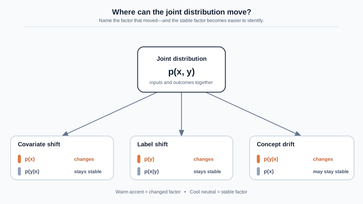
To reason about shift precisely, you need one mental object: the joint distribution p(x, y). It describes the full data-generating process—how inputs x and outputs y co-occur in the world.

The joint distribution can be factored in two useful ways:

• p(x) · p(y|x): the distribution of inputs, times the probability of an output given an input.
• p(y) · p(x|y): the distribution of outputs, times the probability of an input given an output.

Both factorizations describe the same joint distribution. But each type of shift is a claim about which factor moved and which stayed fixed. That is the whole trick: name the moving part, and you know the failure mode.

Let us make this concrete with a running example. Imagine a disease-screening model. The inputs are symptoms; the output is a diagnosis. Now imagine something changes in the world. The question is not just "did something change?" The question is which arrow moved—the arrow from cause to symptom, or the arrow from population to disease prevalence, or the arrow from symptom to diagnosis itself.

Note: The probability notation applies to any supervised problem. The examples that follow use classification because prevalence, thresholds, and class mix are easiest to see there. If your task is regression, translate each shift to its analogue: covariate shift is still input drift, label shift becomes a change in the target distribution, and concept drift becomes a change in the input-to-target mapping you can see in residual patterns.

Covariate Shift: The Inputs Move, the Rules Stay

Covariate shift is the cleanest case. The distribution of inputs p(x) changes, but the relationship between inputs and outputs p(y|x) does not.

Think of a model trained on daytime traffic images and deployed on nighttime roads. The rules of the road did not change. A red light still means stop. But the model never saw headlight glare, dark shadows, or wet asphalt reflecting streetlights. The input distribution moved into territory where the model has no evidence.

Here is why covariate shift hurts even though the input-output relationship is intact: the model only learned from the region of input space it saw during training. When new inputs fall outside that region, the model does not reason—it extrapolates. And extrapolation is where machine learning models make confident, spectacular mistakes.

The detection signal for covariate shift is input statistics drifting—feature means, ranges, category frequencies—while the model's accuracy on a labeled sample may still look reasonable. That last part is the trap. The model can look fine on the labels you have while failing badly on the inputs you do not.

The good news: covariate shift is often fixable. Because the underlying rule did not change, collecting data from the new input region and retraining usually restores performance. You do not need to rethink the problem. You need to show the model the part of the world it missed.

Label Shift: The Outcomes Move, the Symptoms Stay

Label shift, also called prior probability shift, is the mirror image. The distribution of outcomes p(y) changes, but the way each outcome produces its features p(x|y) stays the same.

The direction of causality matters here. Label shift is the correct assumption when the label causes the features—disease causes symptoms, not the reverse. If disease prevalence rises in a population while the symptom profile of each disease is unchanged, you have label shift.

What breaks? Not the learned conditional structure. The model still understands that these symptoms point to this disease. What breaks is the decision threshold you tuned on the old prevalence. If a disease that was rare becomes common, the threshold that made sense at training time now produces the wrong balance of false positives and false negatives.

The detection signal is the predicted class distribution drifting from the training class balance. The response is cheaper than retraining from scratch: recalibrate the threshold or reweight the classes to match the new prevalence. The model's knowledge is still valid. The operating point is not.

Common mistake: A changed predicted class mix is not proof of label shift. Your model's predictions can drift because inputs changed, because the threshold moved, or because the model itself degraded. Label shift is a specific assumption: the true outcome prevalence changed while p(x|y) stayed fixed. Before you reweight or rethreshold, check that assumption against labeled data from the deployment period. If you cannot verify it, treat reweighting as a temporary patch, not a cure.

This is why the factorization matters. If you mistake label shift for covariate shift, you will go recollect data you do not need. If you mistake it for concept drift, you will retrain a model whose conditional structure was never broken.

Concept Drift: The Rules Themselves Change

Concept drift is the hardest case, and the most dangerous. The relationship between inputs and outputs p(y|x) changes, even when the input distribution looks identical.

Consider a recommendation model trained on pre-pandemic browsing behavior. The browsing patterns did not change much—people still visited the same travel sites, watched the same kinds of videos. But the relationship between browsing and purchasing flipped. Someone watching travel content in 2019 might buy plane tickets. The same behavior in March 2020 predicted something entirely different.

This is why concept drift is insidious: input monitoring shows nothing wrong. The features look stable. The model fails silently until labeled feedback reveals that the mapping has changed.

Concept drift comes in two rhythms. Gradual drift is slow decay—a model that gets a little worse each quarter as consumer tastes evolve. Sudden concept change is a policy, regulation, or world event flipping the rule overnight.

The detection signature separates concept drift from covariate shift: accuracy on a labeled sample drops even though feature distributions look stable. If you only monitor inputs, you will miss it entirely. If you only monitor outputs, you will catch it late.

Reading the Evidence: Hypotheses, Not Verdicts

When a deployed model degrades, resist the urge to treat every problem as the same kind of problem. The evidence tells you which shift you are facing—if you collect the right evidence.

Shift type	What changed	Observable signal	Typical response
Covariate shift	Input distribution p(x)	Feature statistics drift; labeled accuracy may hold	Collect data from the new input region; retrain
Label shift	Outcome distribution p(y)	Predicted class mix drifts from training balance	Recalibrate threshold or reweight classes
Concept drift	Input-output mapping p(y|x)	Labeled accuracy drops while inputs look stable	Retrain on recent data; possibly redesign

Here is the catch: these signals are hypotheses, not verdicts. Feature drift can occur without harming performance. Predicted class proportions can change because the inputs changed, not because prevalence did. A performance drop can come from a labeling bug, a pipeline change, or sensor failure—none of which is a distribution shift at all.

So treat the table as a diagnostic starting point, not a proof. The workflow that actually protects you:

1. Detect change. Track input statistics and labeled-sample accuracy over time.
2. Rule out pipeline problems first. Check that the data collection, labeling, and feature-engineering code still behave as they did at training time.
3. Compare labeled outcomes where available. A labeled sample from the deployment period is the ground truth that separates real shift from monitoring noise.
4. Test which shift assumption best explains the evidence. Then choose the response that matches that assumption—and verify it against fresh labeled data.

The common mistake is monitoring only one signal. Input-only monitoring misses concept drift completely. Output-only monitoring misses covariate shift until it has already bitten. You need both—input statistics and labeled-sample accuracy over time—to disambiguate the three cases.

A practical note: you cannot diagnose any of this without a labeled sample from the deployment period. That means investing in a feedback channel—human review, delayed labels, or periodic manual evaluation—even when it feels expensive. Without labels, you can detect that something changed. You cannot tell which part changed.

Monitoring and Responding: Design Around the Boundary You Can See

Once you have evidence for a shift type, the response follows—but only conditionally. Covariate shift calls for recollecting data from the new input region if labeled accuracy actually suffers. Label shift calls for reweighting or rethresholding if you can verify the prevalence change against labeled data. Concept drift calls for retraining on recent data—and sometimes for asking whether the problem itself needs reformulation.

Retraining on recent data is not automatically safe. If that recent data is unrepresentative or contaminated, you can make the model worse. And covariate shift may require no model change at all if performance on a labeled sample remains acceptable. The response follows the measured impact, not the shift label alone.

But be honest about the limits. Some shifts are undetectable in principle. If the mapping from inputs to outputs flips completely while the input distribution stays identical, no monitoring system can distinguish that from a world where nothing changed. The data simply does not contain the evidence. Monitoring catches what is observable; it does not guarantee safety.

For a beginner, the practical takeaway is not to build a full production monitoring system on day one. It is to design experiments and evaluations that assume the world will move. When you evaluate a model, ask: what would break first if the deployment population differed from my training population? Which features would drift? Which base rates could change? What would happen to my threshold if the class balance shifted?

The durable skill is the question, not the tooling. When a deployed model degrades, name the changed component before choosing a fix. Sketch the joint distribution for your own problem. List which shifts are plausible—which inputs could move, which base rates could change, which rules could flip. Then decide what evidence would tell you which one happened.

That habit will not prevent the world from changing. But it will keep you from blaming the model for a world that moved, and it will tell you exactly where to look when the test score stops matching reality.

References

Research updated Sep 8, 2026