Imbalanced Classification: Why Accuracy Can Hide the Failure

A model that predicts "no fraud" for every transaction can score 98% accuracy while catching zero fraud. The number feels trustworthy. It is not. Accuracy is telling you how well you predict the boring majority—not how well you catch the rare event you built the model to find.

The 98% Accuracy Trap

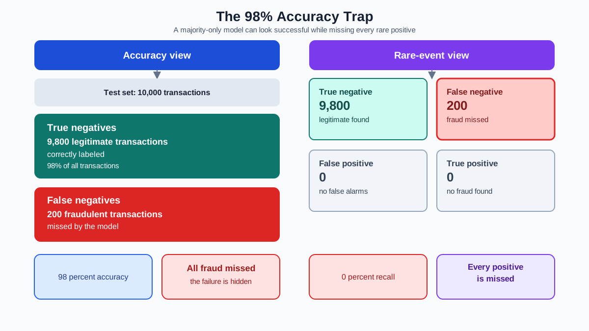
Imagine you are building a fraud detector. Out of every 10,000 transactions, 200 are fraudulent. That is a 2% positive rate, which makes this an imbalanced classification problem.

You train a model. It reports 98% accuracy. Your first reaction is relief. Then you look at what the model actually predicts: it labels every single transaction as legitimate. No fraud alerts, ever. And it still earns that 98%.

Here is the mechanism behind the trap. If 98% of your rows belong to the majority class, a model that always predicts the majority class is correct on 98% of rows by doing nothing. It inherits the majority prevalence as its accuracy score. The model has learned exactly one thing: fraud is rare, so predicting "no fraud" is usually right.

The deeper issue is what accuracy actually measures. Accuracy collapses all four cells of the confusion matrix—true positives, false positives, true negatives, and false negatives—into a single ratio. When true negatives dominate because negatives are common, that one cell swamps everything else. The cells that matter for rare-event detection, the true positives and false negatives, barely move the result. Accuracy rewards the model for correctly predicting the 9,800 legitimate transactions and ignores the fact that it missed all 200 fraudulent ones.

This builds directly on the metric-selection and cross-validation concepts covered elsewhere in the curriculum. What imbalanced classification adds is a warning: the metric itself can be the failure, before you ever tune a model.

Prevalence Is the Hidden Variable

The reason accuracy misleads is not a bug in the formula. It is a missing variable in your interpretation: prevalence, the share of positive examples in your data.

Prevalence changes what a given metric means, independent of how skilled your model is. A random classifier on a balanced dataset expects 50% accuracy. A random classifier on a 2%-prevalence dataset expects roughly 98% accuracy, because guessing the majority class is correct most of the time. The same score means something completely different at different base rates.

This is why metrics that ignore true negatives behave differently from accuracy. Precision and recall never look at the true-negative cell. Recall asks: of the real events present, how many did you catch? Precision asks: of the alerts you raised, how many were real? Both force the model to answer for the rare rows, not the common ones.

Picture the confusion matrix for a constant "predict majority" classifier on a 2%-prevalence problem. The true-negative cell holds 9,800 rows. The other three cells hold 200 rows combined, all of them false negatives. Accuracy sees 9,800 correct answers out of 10,000 and reports success. A metric that ignores true negatives sees 0 real events caught out of 200 and reports total failure.

The mental model to keep: a rare event needs a metric that reacts to the rare rows.

Choose the Metric That Answers Your Question

When accuracy stops being informative, you need metrics that measure the minority class directly. But these metrics are not interchangeable. Each answers a different question, punishes a different error, and depends on prevalence in a different way.

Precision answers: of the alerts you raised, how many were real? If you flag 100 transactions and 40 are actually fraudulent, precision is 0.40. Precision punishes false alarms.

Recall answers: of the real events present, how many did you catch? If 200 fraudulent transactions exist and you flag 40 of them, recall is 0.20. Recall punishes missed events.

F1 is the harmonic mean of precision and recall. The harmonic mean is deliberately harsh: it refuses to let one strong number hide a weak one. A model with precision 0.90 and recall 0.10 gets an F1 of 0.18, not a comfortable average. You cannot cheat F1 by being good at one thing.

Balanced accuracy takes the average of recall on the positive class and recall on the negative class. A constant "predict majority" classifier scores 0.5 on balanced accuracy, no matter how high its plain accuracy reads. That honesty is exactly why balanced accuracy is a useful sanity check on imbalanced problems.

Precision-recall AUC deserves special attention because its baseline tracks prevalence. A random classifier on a 1%-prevalence problem has a PR-AUC of 0.01. A model scoring 0.10 is genuinely ten times better than chance, even though the absolute number looks small. ROC-AUC, by contrast, always baselines at 0.5 regardless of prevalence. That fixed baseline can make a weak model look reassuring on a rare-event problem.

Here is the distinction that matters: precision, recall, F1, and balanced accuracy are thresholded metrics. They describe performance at one specific decision cutoff. PR-AUC and ROC-AUC are ranking metrics. They describe how well the model separates classes across every possible cutoff. A ranking metric tells you whether the model can distinguish fraud from legitimate behavior. A thresholded metric tells you what happens at the operating point you actually deploy.

Which metric should you choose? The answer follows the cost of your errors. If a missed fraud costs thousands of dollars and a false alert costs a customer service email, recall matters more than precision. If false alerts burn your team's trust and get ignored, precision matters more.

If you do not know the costs yet, treat F1 and balanced accuracy as diagnostic summaries, not optimization targets. F1 assumes precision and recall matter equally. Balanced accuracy assumes both classes matter equally. Those are assumptions about your problem, and you should make them consciously rather than inherit them.

Thresholds: The Lever You Are Not Pulling

Most classifiers do not output labels directly. They output a continuous score, and something else decides where the cutoff sits. That something else is usually a default: 0.5.

The default threshold encodes an assumption. It assumes balanced classes and equal costs for false positives and false negatives. Rare-event problems rarely satisfy either condition.

Lowering the threshold catches more real events at the price of more false alerts. At a 0.5 threshold, your fraud model might catch 40% of fraud with very few false alarms. Drop the threshold to 0.1 and you might catch 80% of fraud—but now you are also flagging legitimate transactions that look vaguely suspicious.

Threshold choice should follow the cost structure of your problem, not a fixed convention. If a missed fraudulent transaction costs you real money and a false alert costs a quick review, you want the threshold low enough to catch most fraud. If every false alert costs an expensive investigation, you want it higher.

The precision-recall curve is your tool here. It shows the trade directly: as recall climbs, precision falls. Pick the operating point where the trade matches your costs. Some practitioners use a simple cost-based rule: choose the threshold where the expected cost of false negatives and false positives is minimized, given your estimated costs for each.

A common mistake is treating the threshold as fixed while only tuning the model. The model and the threshold are two separate decisions. You can ship the same model with a different threshold and get a completely different operational behavior.

One caution: a classifier's score is a ranking signal, not necessarily a trustworthy probability. The threshold converts that score into labels. You can tune the threshold without retraining the model, but you should not assume the score itself is calibrated to true event rates.

Sampling and Class Weights: Fixing the Data or the Loss

When beginners hit imbalanced classification, the first instinct is to rebalance the data. That instinct is reasonable, but it needs precision about what each technique actually does.

Oversampling duplicates minority-class rows until the classes look balanced. Undersampling discards majority-class rows. Both change the training distribution so the model sees more minority examples per batch.

SMOTE goes further: instead of duplicating existing minority samples, it creates synthetic ones by interpolating between a minority point and its neighbors. The new samples are plausible variations rather than exact copies.

Class weights take a different route. Instead of changing the data, they change the loss function so mistakes on the minority class cost more. The model still sees the original distribution, but it learns that missing a fraud case is more expensive than missing a legitimate transaction.

Here is the critical rule: resample or reweight only the training folds, never the test set. If you balance the entire dataset before splitting, your test set no longer reflects real-world prevalence, and every metric you compute on it is optimistic fiction. The test set must look like the world the model will actually operate in.

Rebalancing can raise recall while lowering precision. That trade is often the point: you are trading some false alarms for catching more real events. If the cost structure justifies it, the trade is a win.

One honest warning: if the minority class is genuinely hard to separate—the features simply do not distinguish fraud from legitimate behavior—no resampling technique rescues it. Sampling changes the training distribution. It does not create signal where none exists.

Validation That Does Not Lie

Cross-validation already taught you the value of stratification. Imbalanced classification makes stratification non-negotiable.

A random split on a rare class can produce a validation fold with almost no positive examples. If your positive rate is 2% and you draw a fold of 1,000 rows, you might get 15 positives in one fold and 25 in another. The model trains on uneven views of the minority class, and your performance estimate wobbles with the luck of the split.

Stratified folds keep the minority-class share consistent across training and validation. Each fold sees roughly the same prevalence, so each fold produces a comparable estimate of minority-class performance.

Two more practices matter. First, evaluate on the real-world prevalence, not an artificially balanced test set. Second, report the minority-class metrics per fold, not just the pooled average. If recall is 0.80 in four folds and 0.40 in one fold, the pooled number hides a stability problem you need to see.

The threshold needs the same discipline. Threshold selection is part of model selection. Choose the operating point using training folds or cross-validation, lock it, and then evaluate it once on an untouched test set. If you tune the threshold on the test set, your reported performance is inflated by your own search.

A Decision Rule for Your Next Imbalanced Problem

When you hit an imbalanced classification problem, work through this sequence:

1. Check prevalence. Know the positive rate before you choose any metric.
2. Build the majority-class baseline. A constant "predict majority" model gives you the accuracy floor. Any real model must beat it on the metrics that matter.
3. Choose the metric that matches error cost. Missed events expensive? Optimize recall, possibly with a minimum acceptable precision. False alerts expensive? Optimize precision, possibly with a minimum recall target. Unsure? Use balanced accuracy as a diagnostic summary, not a final target.
4. Tune the threshold. Treat 0.5 as a starting point, not a rule. Use the precision-recall curve to find the operating point that matches your costs. Lock the threshold before touching the test set.
5. Decide if sampling or weights add value. Try class weights first—they are simpler and do not risk test-set leakage. Add resampling only if the model still ignores the minority class.

This toolkit works for rare events with meaningful cost asymmetry: fraud detection, disease screening, equipment failure prediction, churn identification. It is the right tool when the event you care about is uncommon and the cost of missing it is not symmetrical with the cost of a false alarm.

It is the wrong tool when the minority class is too small to learn from at all, or when the real bottleneck is feature quality. If you have 50 positive examples across 40 features, no sampling strategy manufactures the information you lack. Collect more data or engineer better features first.

The durable mental model: accuracy answers "how often am I right overall." It does not answer "how well do I catch the rare thing I built this for." Run this sequence on your own data. Check prevalence, build the majority baseline, pick the metric that matches your costs, and tune the threshold before you reach for sampling. The model that looks broken under honest metrics is often the one that actually works.

References

Research updated Sep 8, 2026