
Hierarchical Clustering Linkages: Define Distances and Work Through Merges
Change one parameter, get a different tree. Same points, same distance metric, same greedy loop — yet the dendrogram reorganizes itself. That parameter is…

Key topics
Change one parameter, get a different tree. Same points, same distance metric, same greedy loop — yet the dendrogram reorganizes itself. That parameter is the linkage, and it decides what "closest clusters" actually means.
The Merge Rule Is the Whole Algorithm
Agglomerative clustering is almost embarrassingly simple. Start with every point as its own cluster. Find the two closest clusters. Merge them. Repeat until one cluster remains. That is the entire loop.
The catch is buried in the phrase "two closest clusters." When both objects are single points, distance is unambiguous: you measure from one coordinate to the other. But once clusters contain multiple points, "the distance between cluster A and cluster B" has no single obvious answer. Do you measure the closest pair? The farthest pair? The average across all pairs? Each choice is a different linkage function, and each one produces a different tree from identical data.
Fix notation before going further. Let points be , and let be the distance between two individual points. Let and be clusters — sets of points. A linkage function returns a single scalar: the distance between those two clusters. The algorithm is then:
- Compute for every pair of current clusters.
- Merge the pair with the smallest .
- Update the distance from the new cluster to every other cluster.
- Repeat until one cluster remains.
Linkage changes only step 1. The loop, the greedy selection, and the merge structure stay fixed. That is why swapping the linkage parameter feels like swapping the data: the rule that decides "closest" has changed, so every subsequent merge decision changes with it.
If you already know when to reach for hierarchical clustering over K-means, this article assumes that choice is made. The question here is narrower and more mechanical: given that you are building a tree, how is the tree actually built?
Knowledge check
Check your understanding
Answer this question before you continue.
Single, Complete, and Average Linkage
Three classic linkages differ only in which cross-cluster pair they consult.
Single linkage takes the minimum:
Only the closest pair matters. Two clusters are "close" if any two of their members are close. This lets clusters grow by chaining: point by point, each new point only needs to be near one existing member, so a long snaking cluster can form across a region that is not compact at all.
Complete linkage takes the maximum:
Now the farthest pair governs. Two clusters are "close" only if every point in one is close to every point in the other. This pushes toward compact, roughly equal-diameter clusters, because a single distant point inflates the distance and blocks the merge.
Average linkage (also called UPGMA) takes the mean over all cross pairs:
Every cross-cluster pair contributes. This is a compromise: less sensitive to a single outlier than complete linkage, less prone to chaining than single linkage.
The min/max/mean distinction is not cosmetic. Each formula encodes a different assumption about what "close clusters" means, and that assumption propagates through every merge. SciPy exposes these directly as single, complete, average, weighted, centroid, median, and ward methods on scipy.cluster.hierarchy.linkage, so the formulas map onto callable functions rather than abstractions.
Knowledge check
Check your understanding
Answer this question before you continue.
Ward's Method: Minimize the Variance You Add
Ward linkage does not pick a representative pair at all. It asks a different question: which merge adds the least variance?
Define the within-cluster sum of squared distances to the centroid. Ward chooses the merge that produces the smallest increase in the total sum of squares across all clusters. For two clusters and with centroids and , the increase in sum of squares from merging them is:
Read the formula as two coupled terms. The squared centroid distance is the obvious one: far-apart clusters cost more to merge. The size factor is the subtle one. For a fixed centroid separation, it grows with the combined size of the two clusters, so merging two large clusters is more expensive than merging a large cluster with a small one. Ward is not "biased toward equal sizes" in isolation — it is minimizing the full cost, and the size factor is one of two inputs that determine that cost. The practical tendency toward balanced clusters emerges from how the two terms interact across the whole dataset, not from the size factor alone.
Warning: Ward's variance argument assumes squared Euclidean distance. Pair it with a non-Euclidean metric and the interpretation breaks; the formula still runs, but "minimizing variance" no longer describes what it does.
Centroid and median linkage also use centroids, but they can produce non-monotonic dendrograms — a merge that happens at a lower height than an earlier merge. That makes the tree harder to read, because branch height no longer increases monotonically as you move up.
Knowledge check
Check your understanding
Answer this question before you continue.
Work Through Five Points by Hand
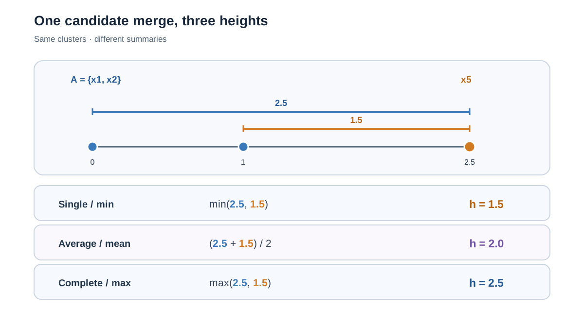
Abstraction earns its keep only when you can reproduce it. Take five points on a line: , , , , . Use absolute distance.
The pairwise distance matrix:
| 0 | 1 | 5 | 6 | 2.5 | |
| 1 | 0 | 4 | 5 | 1.5 | |
| 5 | 4 | 0 | 1 | 2.5 | |
| 6 | 5 | 1 | 0 | 3.5 | |
| 2.5 | 1.5 | 2.5 | 3.5 | 0 |
The global minimum is 1, appearing twice: and . The first merge is identical under every linkage because all clusters are singletons — there is no ambiguity yet. Merge and into , and and into .
Now the linkages diverge. Compute the distance from each existing cluster to the remaining singleton :
- Single:
- Complete:
- Average:
And from to :
- Single:
- Complete:
- Average:
Now compare the candidate merges at this stage. Under single linkage, the smallest available distance is – at 1.5, so single linkage merges with next. Under complete linkage, the smallest available distance is – at 2.5, so complete linkage also merges with next — but at a different height. Under average linkage, the smallest is again – at 2.0.
The merge pair is the same here, but the merge height differs: 1.5, 2.5, and 2.0. That height difference is what reshapes the dendrogram. To force a different merge pair, move closer to . Set :
- Single: ;
- Complete: ;
- Average: ;
Now every linkage prefers –, but the gap between the two candidates differs sharply. Under single linkage, the gap is . Under complete linkage, it is . Under average, it is . The gaps happen to match here because the points are collinear. On real data with two-dimensional geometry, the gaps diverge, and the merge order can flip.
The lesson is not the specific numbers. It is that the ordering and height of merges, not just the final partition, is what changes. Each merge height becomes a branch height in the dendrogram, so a different merge order produces a visibly different tree.
Knowledge check
Check your understanding
Answer this question before you continue.
How Linkage Reshapes the Dendrogram
Once you have traced a few merges, the dendrogram stops being a picture and becomes a fingerprint.
- Single linkage produces long, straggly trees with late, high merges. That shape is the signature of chaining: clusters absorb nearby points one at a time, and the final merge happens only when everything is already connected.
- Complete linkage produces more balanced trees with tighter merge heights, but a single outlier can distort the whole structure by inflating every distance it touches.
- Average linkage sits between the two and is often the least surprising default when clusters are roughly similar in size.
- Ward produces the most balanced trees and is the common default in scikit-learn's
AgglomerativeClustering, but its balance reflects the variance objective, not the data.
Tip: A suspiciously chain-like dendrogram is a linkage signal, not necessarily a data signal. Before concluding your data has an elongated structure, check whether single linkage is manufacturing it.
Choosing a Linkage Without Fooling Yourself
The formulas are settled. The judgment is not.
Match the linkage to the geometry you expect. If you expect elongated or non-convex clusters, single linkage can find them — but it will also chain noise into the same cluster. If you expect compact, similar-sized groups, Ward or complete linkage is a safer start.
Scale before you choose. Feature scaling matters more than linkage choice in many datasets. Features on different units will dominate the distance matrix before any linkage formula runs, and no linkage can recover from a distance matrix that already encodes the wrong geometry.
Know how each linkage fails. Complete and Ward are pulled by extreme points. Single linkage can bridge two genuinely separate clusters through one stray point. Average linkage is the most forgiving of the three, which is part of why it is a common default.
Do not treat a clean dendrogram as validated structure. Linkage is one of several degrees of freedom, alongside metric, scaling, and cut height. A tidy tree is a tidy tree; it is not proof that the groups are real.
Know when to skip this family. Very large datasets, or problems where you need a single flat partition and the hierarchy adds no interpretive value, are better served by a different method.
The habit worth building: before you trust any dendrogram, name the linkage, the metric, and the scaling. Those three choices — not the data alone — produced the tree you are reading.
Run the five-point example through single, complete, average, and Ward linkage in SciPy. Compare the merge heights. The fastest way to internalize how much the linkage rule controls the result is to watch four different trees grow from the same five numbers.
Knowledge check
Final check
Finish the article by checking the ideas you just learned.
References
Build stronger machine learning foundations
Use structured resources to connect theory, scikit-learn workflows, and evaluation practice.


