
Experiment With Gradient Boosting: Learning Rate, Trees, and Validation
A single accuracy number tells you almost nothing. A controlled experiment tells you whether that number means anything at all.

Key topics
A single accuracy number tells you almost nothing. A controlled experiment tells you whether that number means anything at all.
You already know how gradient boosting works: trees are added one at a time, each fit to the error the current ensemble has not yet explained, then scaled by a learning rate and added into the sum. What you probably do not have yet is a way to feel those controls. You change learning_rate, the score moves, and you have no idea whether the movement came from the knob you turned or from noise.
The fix is not a better model. It is a better experiment. Freeze one split. Change one knob at a time. Read the gap between training and validation, not the score alone. By the end of this tutorial you will have a reusable harness you can point at any boosting configuration, and a mental model for why each configuration behaves the way it does.
What This Experiment Is Actually Testing
Before any code, let's set the contract.
The task is binary classification on a synthetic dataset built with make_classification and a fixed random_state, so the data itself is reproducible. We create one stratified train/validation split, once, with a fixed seed, and reuse it for every configuration. That single split is the control that makes every later comparison meaningful.
Two knobs are under test: learning_rate and max_depth. Everything else stays at scikit-learn defaults so the comparison stays honest.
Success here is diagnostic, not numeric. The code runs end to end, and you can say whether a configuration shows a train/validation gap. There is no winner to declare. If you find yourself hunting for the best score, you have drifted off the point.
Note: This assumes you already know that boosting fits trees sequentially to remaining error, and that training, validation, and test sets have distinct jobs. If either is fuzzy, revisit those first — the rest of this article leans on them.
Build the Fixed Split and a Baseline Fit
Let's get runnable code on screen fast. Imports, dataset, split, baseline model, first numbers.
import numpy as np
import pandas as pd
import matplotlib.pyplot as plt

from sklearn.datasets import make_classification
from sklearn.model_selection import train_test_split
from sklearn.ensemble import GradientBoostingClassifier
from sklearn.metrics import accuracy_score

# Reproducible synthetic data
X, y = make_classification(
    n_samples=1200,
    n_features=12,
    n_informative=6,
    n_redundant=3,
    random_state=42,
)

# One stratified split, created once, reused everywhere
X_train, X_val, y_train, y_val = train_test_split(
    X, y, test_size=0.25, stratify=y, random_state=42
)

print("Train class balance:", np.bincount(y_train) / len(y_train))
print("Val class balance:  ", np.bincount(y_val) / len(y_val))
Printing the class balance on both sides is not ceremony. It confirms stratify=y actually did its job. If the two distributions diverge, your split is lying to you before you have fit a single model.
Now the baseline:
baseline = GradientBoostingClassifier(random_state=42)
baseline.fit(X_train, y_train)

train_acc = accuracy_score(y_train, baseline.predict(X_train))
val_acc = accuracy_score(y_val, baseline.predict(X_val))

print(f"Train accuracy: {train_acc:.4f}")
print(f"Val accuracy:   {val_acc:.4f}")
print(f"Gap:            {train_acc - val_acc:.4f}")
A plausible run looks like this:
Train accuracy: 1.0000
Val accuracy:   0.9200
Gap:            0.0800
Your exact numbers will differ with scikit-learn version and seed. That is fine. The baseline is not a model to beat — it is the reference point every later configuration gets compared against.
Knowledge check
Check your understanding
Answer this question before you continue.
Turn the Fit Into a Configuration Table
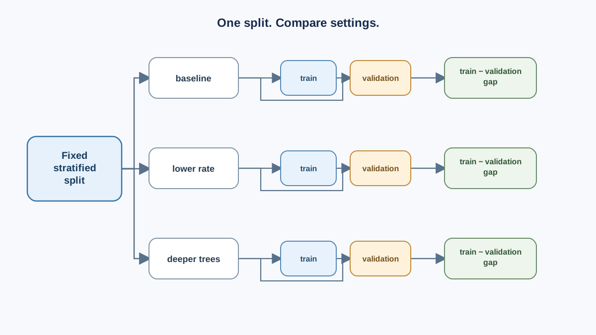
One-off fits are how you end up eyeballing single runs and calling it analysis. Let's convert the fit into a loop that records train and validation metrics per configuration.
def evaluate(config, X_train, y_train, X_val, y_val):
    model = GradientBoostingClassifier(random_state=42, **config)
    model.fit(X_train, y_train)
    train_acc = accuracy_score(y_train, model.predict(X_train))
    val_acc = accuracy_score(y_val, model.predict(X_val))
    return {
        "config": config,
        "train_acc": round(train_acc, 4),
        "val_acc": round(val_acc, 4),
        "gap": round(train_acc - val_acc, 4),
    }

configs = [
    {"learning_rate": 0.1, "max_depth": 3},   # baseline defaults
    {"learning_rate": 0.01, "max_depth": 3},  # lower rate
    {"learning_rate": 0.5, "max_depth": 3},   # higher rate
    {"learning_rate": 0.1, "max_depth": 1},   # shallower trees
    {"learning_rate": 0.1, "max_depth": 6},   # deeper trees
]

results = pd.DataFrame([evaluate(c, X_train, y_train, X_val, y_val) for c in configs])
print(results.to_string(index=False))
The split lives outside the loop and gets passed in. This is the single most common place readers accidentally re-split and destroy comparability. If you find yourself calling train_test_split inside evaluate, stop.
The table is the artifact. Read it as a set of patterns to check, not guaranteed outcomes:
| Row | What changed | Pattern to look for |
|---|---|---|
| Lower rate | Each tree contributes less | Train and val may both sit lower; the gap often narrows |
| Higher rate | Each tree contributes more | Train may climb faster; val may lag or stall |
| Deeper trees | Each tree partitions finer | Train may approach 1.0; the gap may widen |
| Shallower trees | Each tree is a weak stump | Both scores may drop; the gap often stays narrow |
On a single synthetic split, accuracy can stay flat or move irregularly. Treat each row as a hypothesis your run either supports or contradicts — not a rule the data has to obey.
Knowledge check
Check your understanding
Answer this question before you continue.
Reading the Table Through Sequential Additive Fitting
Numbers become a mental model only when you can explain them through the mechanism.
Each tree is fit to the remaining error of the current ensemble, then scaled by learning_rate and added. The ensemble is a sum, not a replacement. Every observation below falls out of that one fact.
Lower learning rate. Each tree contributes less to the sum, so the model needs more trees to reach the same fit. It is slower to overfit and slower to converge. On the table, both train and validation accuracy often sit lower than the baseline — not because the model is worse, but because it has not finished climbing.
Higher learning rate. Each tree contributes more. The ensemble reaches high training fit in fewer stages and can overshoot into a wider train/validation gap. Training accuracy shoots up; validation accuracy may stall or dip.
Deeper max_depth. Each individual tree can carve finer partitions, so the ensemble can memorize training detail faster. This is the same overfitting story as a single deep decision tree, now multiplied across stages. Training accuracy climbs toward 1.0 while validation plateaus.
Shallower trees. A depth-1 stump is a complexity ceiling per stage. The ensemble can still fit, but it has to do it in smaller, more additive steps. Both scores drop, and the gap usually narrows.
Common mistake: Tuning
n_estimatorswhile thinking you are tuning tree complexity.n_estimatorsis how many trees get added sequentially.max_depthis how complex each one is. They are different axes, and confusing them is how people conclude boosting "does not help."
One honest boundary: this experiment shows behavior on one synthetic dataset with one split. It does not establish a universal best learning rate. It establishes a method for finding out.
Knowledge check
Check your understanding
Answer this question before you continue.
Plot Validation Score Against Estimator Count
The table gives you a snapshot. The staged curve gives you the trajectory.
staged_predict returns predictions after each boosting stage, so you can compute validation accuracy as trees accumulate.
def staged_val_curve(config, X_train, y_train, X_val, y_val):
    model = GradientBoostingClassifier(random_state=42, **config)
    model.fit(X_train, y_train)
    return [
        accuracy_score(y_val, y_pred)
        for y_pred in model.staged_predict(X_val)
    ]

plt.figure(figsize=(9, 5))
for config in [
    {"learning_rate": 0.01, "max_depth": 3, "n_estimators": 500},
    {"learning_rate": 0.5,  "max_depth": 3, "n_estimators": 500},
]:
    curve = staged_val_curve(config, X_train, y_train, X_val, y_val)
    plt.plot(range(1, len(curve) + 1), curve, label=str(config))

plt.xlabel("Number of estimators")
plt.ylabel("Validation accuracy")
plt.legend()
plt.tight_layout()
plt.show()
What to look for:
- Where each curve peaks. That is the point where more trees stop helping.
- Whether it plateaus. A flat curve means the ensemble has saturated.
- Whether it turns downward. A sustained decline while training accuracy keeps climbing is evidence consistent with overfitting. A single dip is not — inspect the actual run before assigning a cause.
Compare the two lines on the same axes. The low-rate curve typically rises more slowly and keeps improving longer. The high-rate curve rises fast and can peak early, then sag. That shape is the learning-rate/tree-count tradeoff made visible.
And note the cost: more estimators means more fitting time. The low-rate/high-count setting is not free.
Three Mistakes That Break the Experiment
Split inconsistency. Re-splitting inside the loop, or forgetting stratify, produces rows that are not comparable. The symptom is validation scores that jump around for reasons unrelated to the knob you changed. The fix is to build the split once and pass it in.
Overly complex trees. A large max_depth on a small dataset drives training accuracy toward 1.0 while validation stalls or drops. The symptom is a wide, growing gap. Cap the depth and re-read the table.
Confusing estimator count with tree depth. n_estimators is how many trees are added sequentially. max_depth is how complex each one is. The symptom is tuning the wrong knob and concluding boosting does not help. Before you change anything, name which axis you are changing.
A fourth, quieter one: changing two knobs at once and attributing the result to one of them. If you change learning_rate and max_depth in the same run, you have learned nothing about either.
Knowledge check
Check your understanding
Answer this question before you continue.
Follow-Up: Lower Learning Rate, More Trees
Now change exactly two things: reduce learning_rate and increase n_estimators proportionally. Keep max_depth, the split, and random_state identical. Use the baseline configuration as your fixed reference so the comparison stays clean.
original = {"learning_rate": 0.1, "max_depth": 3, "n_estimators": 100}
slower   = {"learning_rate": 0.02, "max_depth": 3, "n_estimators": 500}

for name, config in [("original", original), ("slower", slower)]:
    curve = staged_val_curve(config, X_train, y_train, X_val, y_val)
    plt.plot(range(1, len(curve) + 1), curve, label=name)

plt.xlabel("Number of estimators")
plt.ylabel("Validation accuracy")
plt.legend()
plt.tight_layout()
plt.show()
Compare peak validation score and the shape of the curve against the original setting. The interpretation rule is simple: if the lower-rate run matches or beats the original validation score, you have paid for it in fitting time. Decide whether that trade is worth it for your problem.
Treat any "best" row from your table as a provisional observation on this split, not a winner. The same validation set you inspected to build the table is now the one you are reading again — repeated inspection turns it into a soft training signal. If you want a real selection decision, hold out a separate test set or use cross-validation on a fresh split.
Then change one more thing deliberately. Predict the outcome before you run it. Prediction-then-check is how the mental model gets tested — and how you find out which parts of it are still wrong.
What You Now Own
You did not build a tuned model. You built a reusable experiment harness: a fixed split, one knob at a time, the train/validation gap as the primary signal, and staged curves to see where performance turns.
That harness is the real deliverable. Point it at any future boosting run and the diagnostic clues hold: a wide gap suggests memorization, low scores on both sides suggest underfitting, and a sustained validation decline while training keeps improving suggests more trees are hurting you. Each is a clue to investigate, not a verdict — one split cannot prove a universal rule.
The natural next step is to extend the same harness to other controls — subsample for stochastic boosting, min_samples_leaf for leaf-level regularization — or to run a different ensemble family under the identical split and compare the shapes. Same split, same discipline, new question. That is how the mental model compounds.
Knowledge check
Final check
Finish the article by checking the ideas you just learned.
References
Build stronger machine learning foundations
Use structured resources to connect theory, scikit-learn workflows, and evaluation practice.


