
A Decision Tree Experiment: Inspect Splits and Observe Overfitting
A decision tree can score 100% on the data it was trained on and still be wrong about almost everything else. That gap is not a bug. It is the lesson.

Key topics
A decision tree can score 100% on the data it was trained on and still be wrong about almost everything else. That gap is not a bug. It is the lesson.
This is a short, runnable experiment. The whole point is to make that gap appear on purpose, then shrink it by turning one dial: how deep the tree is allowed to grow. By the end, you will have a small script that fits a DecisionTreeClassifier at several depths and prints training accuracy next to validation accuracy, so you can watch the two numbers pull apart.
I like this experiment because it is the cheapest way I know to feel overfitting in your hands instead of reading about it. You fit a model, look inside it, change one number, and the output tells you whether you understood.
What This Experiment Will Show You
Before any code, here is what "done" looks like:
- A script that fits a decision tree at several
max_depthvalues. - A table with two columns: training accuracy and validation accuracy.
- A visible pattern: training accuracy climbs toward 1.0, while validation accuracy rises, peaks, and then falls.
That falling tail is the thing you are hunting. When you see it, you have observed overfitting directly rather than taking someone's word for it.
You will need Python with scikit-learn, NumPy, and pandas installed. matplotlib is optional, and only if you want to look at a picture of the tree.
Two assumptions carry over from earlier reading. First, you already know that a tree splits data into regions and that depth controls how many splits stack up. Second, you have seen the idea of a train/validation boundary. We are not re-deriving impurity here, and we are not re-teaching why validation exists. We are going to use both.
Why max_depth? Because it is the single most direct complexity control on a tree. It is one integer, it is easy to reason about, and its effect on the model is immediate. If you want one dial to turn while you watch generalization move, this is the dial.
Set Up the Data and the Split
We will use a small, familiar dataset so you can reason about the features by name instead of staring at anonymous columns. The Iris dataset ships with scikit-learn and is small enough to fit in your head.
import numpy as np
import pandas as pd
from sklearn.datasets import load_iris
from sklearn.model_selection import train_test_split

iris = load_iris()
X = pd.DataFrame(iris.data, columns=iris.feature_names)
y = pd.Series(iris.target, name="species")

X_train, X_val, y_train, y_val = train_test_split(
    X, y, test_size=0.3, random_state=42, stratify=y
)

print("train shape:", X_train.shape, "validation shape:", X_val.shape)
print("class balance (train):")
print(y_train.value_counts(normalize=True).round(3))
The random_state=42 matters more than it looks. Without a fixed seed, scikit-learn can break ties between equally good splits differently on each run, and your numbers will drift between executions. Fix the seed once, and every later comparison is fair.
Each split has one job. The training data fits the tree. The validation data judges it. That is the whole contract, and it is worth saying plainly because it is easy to violate by accident.
Warning: Do not use the validation set to pick your depth and then report that same validation score as your final result. The moment validation influences a decision, it stops being a clean judge. If you want an honest final number, hold back a separate test set, or use cross-validation on the training data to choose the depth.
Printing the shapes and class balance first is not busywork. If one class dominates, plain accuracy will flatter your model later, and you want to know that before you start trusting scores.
Knowledge check
Check your understanding
Answer this question before you continue.
Fit One Tree and Read Its Structure
Start with an unconstrained tree. No depth limit, no minimum leaf size. Let it grow until it is satisfied.
from sklearn.tree import DecisionTreeClassifier
from sklearn.metrics import accuracy_score

tree = DecisionTreeClassifier(random_state=42)
tree.fit(X_train, y_train)

train_acc = accuracy_score(y_train, tree.predict(X_train))
val_acc = accuracy_score(y_val, tree.predict(X_val))

print(f"train accuracy: {train_acc:.3f}")
print(f"validation accuracy: {val_acc:.3f}")
print("nodes:", tree.tree_.node_count)
print("depth:", tree.get_depth())
On a dataset this small and clean, you will likely see training accuracy at or near 1.000 and validation accuracy noticeably lower. That is the gap, and it is the entire subject of this article.
Now look inside the tree. A fitted tree is not a black box; it is a data structure you can read.
from sklearn.tree import plot_tree
import matplotlib.pyplot as plt

plt.figure(figsize=(12, 6))
plot_tree(tree, max_depth=2, feature_names=iris.feature_names,
          class_names=iris.target_names, filled=True, fontsize=9)
plt.show()
Notice the max_depth=2 in the plotting call. That is deliberate. A full-depth tree on Iris is a wall of boxes, and a wall of boxes teaches nothing at a glance. Truncating the picture to two levels keeps it readable while still showing you the top splits, the thresholds, and the class counts in each node.
To see a prediction as a sequence of comparisons rather than a magic number, walk one sample down the tree:
sample = X_val.iloc[[0]]
path = tree.decision_path(sample)
leaf = tree.apply(sample)

print("predicted class:", iris.target_names[tree.predict(sample)[0]])
print("leaf node id:", leaf[0])
print("nodes visited:", path.indices)
Every prediction is a chain of "is this feature less than or equal to that threshold?" questions, ending at a leaf that holds a class distribution. The tree does not know anything you cannot read off its nodes.
Here is the mechanism behind the gap: an unconstrained tree keeps splitting until its leaves are pure, meaning every training row in a leaf shares a label. Pure leaves are perfect on training data by construction. They are also where the memorization lives.
Knowledge check
Check your understanding
Answer this question before you continue.
Sweep max_depth and Watch the Gap
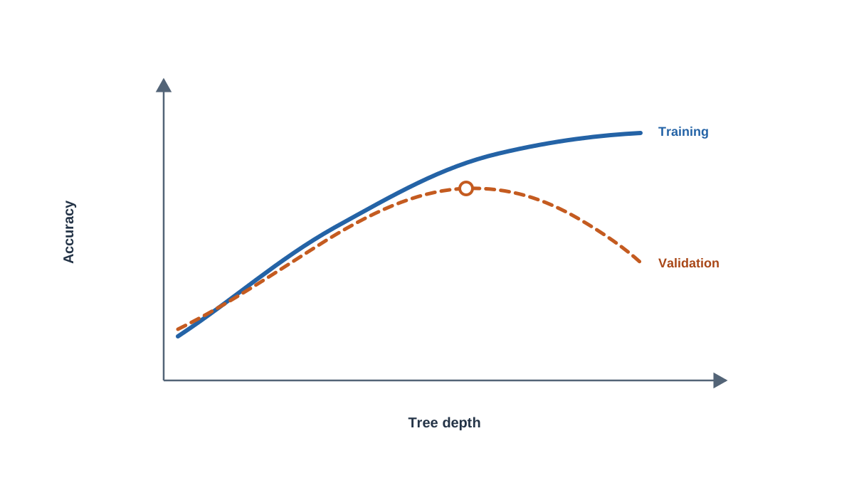
Now the core experiment. Fit a fresh tree at each depth, and record both scores side by side.
results = []

for depth in range(1, 16):
    model = DecisionTreeClassifier(max_depth=depth, random_state=42)
    model.fit(X_train, y_train)
    results.append({
        "max_depth": depth,
        "train_acc": accuracy_score(y_train, model.predict(X_train)),
        "val_acc": accuracy_score(y_val, model.predict(X_val)),
    })

df = pd.DataFrame(results)
df["gap"] = df["train_acc"] - df["val_acc"]
print(df.round(3).to_string(index=False))
Your exact numbers will depend on the split, but the shape is what matters. It looks roughly like this:
| max_depth | train_acc | val_acc | gap |
|---|---|---|---|
| 1 | 0.67 | 0.64 | 0.03 |
| 2 | 0.95 | 0.91 | 0.04 |
| 3 | 0.98 | 0.93 | 0.05 |
| 5 | 1.00 | 0.91 | 0.09 |
| 10 | 1.00 | 0.89 | 0.11 |
| 15 | 1.00 | 0.89 | 0.11 |
Read the columns in order. Training accuracy rises and then pins at 1.000. Validation accuracy rises, peaks somewhere in the middle, and then turns down. The gap widens as depth increases.
That turning point is a pattern that suggests overfitting on this split: the tree stops capturing signal and starts fitting noise. The mechanism is simple arithmetic. Each additional level roughly doubles the number of regions the tree can carve out. A shallow tree can only draw a few broad boundaries. A deep tree can isolate smaller and smaller groups of training rows until each group is its own private leaf. When a leaf contains two or three training examples, it has learned those examples, not the pattern behind them.
Keep random_state=42 fixed across the whole sweep. If you let it vary, differences in the table could come from split randomness rather than from depth, and you would be reading noise as signal.
Knowledge check
Check your understanding
Answer this question before you continue.
Read the Curve, Not the Single Number
The best depth is the one with the best validation score, not the best training score. Training accuracy is a fit report. It tells you how well the tree memorized. It does not tell you whether the tree is any good.
Two signatures are worth memorizing:
- Large train-minus-validation gap: overfitting. The model fits the training data much better than new data.
- Both scores low: underfitting. The model is too simple to capture the pattern at all.
There is a trap in reading these curves. With a small validation set, one lucky depth can look best by chance. A single spike in the validation column is weak evidence. A flat plateau where several neighboring depths score similarly is much more trustworthy, because it means the result is not sensitive to the exact depth you picked.
That is also why the downturn in the table is a clue, not a verdict. A single split gives you one estimate of the curve. To check whether the peak is stable, run the same sweep with cross-validation on the training data and see whether the best depth moves. If it does, the exact turning point was partly noise. If it holds, you have a pattern worth trusting.
Depth is also not your only control. min_samples_leaf and min_samples_split limit how finely a node may be carved, and they often produce smoother generalization behavior than depth alone. A tree with min_samples_leaf=5 cannot create a leaf holding two rows, no matter how deep it goes.
Knowledge check
Check your understanding
Answer this question before you continue.
When the Experiment Misleads You
The experiment is simple, which means it is easy to fool yourself. Here are the failure modes I see most often.
Non-determinism. Without a fixed random_state, ties between equally good splits get broken differently on each run. Your table shifts, and you chase a difference that was never real.
Leakage. If a feature encodes the label, or was computed using the full dataset before you split, validation accuracy will look excellent and mean nothing. The tree is reading the answer key.
Class imbalance. Plain accuracy can look high while the tree quietly ignores the minority class. Check per-class behavior before you trust the headline number.
Tiny validation sets. A handful of rows makes every accuracy jump look dramatic. Always report the number of validation samples next to the score, so the reader knows how much weight the number can carry.
High-dimensional data with few rows. Trees overfit easily when features outnumber samples. On data like that, the depth sweep will turn down earlier than you expect, and the peak validation score will be lower.
Common mistake: Treating the best validation score as a property of the algorithm. It is a property of this dataset, this split, and this seed. Change any of them and the winning depth can move.
Your Next Experiment: Change a Second Dial
You have one dial working. Now add a second and watch how the curve responds.
Re-run the sweep with min_samples_leaf set to a few values, and compare the shape of the validation curve against the depth-only version:
for leaf_size in [1, 3, 5, 10]:
    scores = []
    for depth in range(1, 16):
        model = DecisionTreeClassifier(
            max_depth=depth, min_samples_leaf=leaf_size, random_state=42
        )
        model.fit(X_train, y_train)
        scores.append(accuracy_score(y_val, model.predict(X_val)))
    best = max(scores)
    print(f"min_samples_leaf={leaf_size:>2}  best val_acc={best:.3f}")
Then try two more modifications. Swap the single validation split for cross-validation and see whether the best depth moves. And compare your chosen tree against a trivial baseline that always predicts the majority class, so you learn to ask whether the model beats doing nothing at all.
Record two numbers when you finish: the winning depth and the gap at that depth. That pair is the honest summary of the experiment. A single accuracy figure without its gap is incomplete evidence, and you should treat it that way.
The same tension you just watched — complexity up, training fit up, generalization eventually down — is what drives the ensemble methods that come next. A random forest does not escape this tradeoff. It manages it by combining many constrained trees instead of trusting one deep one. Run the sweep once more with min_samples_leaf, and you will have the intuition you need to understand why.
Knowledge check
Final check
Finish the article by checking the ideas you just learned.
References
Build stronger machine learning foundations
Use structured resources to connect theory, scikit-learn workflows, and evaluation practice.


