Derive the EM Algorithm for Gaussian Mixture Models

You can write the Gaussian mixture density in a single line. The trouble starts the moment you take the log.

For a single Gaussian, the log-likelihood is a clean sum of quadratic terms, and setting the gradient to zero hands you closed-form maximum likelihood estimates for the mean and covariance. For a mixture, the log lands on a sum inside the log, and the derivative stops cooperating. That is the wall this article climbs. The fix is not a cleverer optimizer. It is a missing variable.

If you already know what a Gaussian mixture is — components, weights, soft membership — you have the intuition. What you likely do not yet have is the mechanism: why the observed-data likelihood resists direct maximization, how a latent assignment variable splits the problem into two tractable pieces, and where each closed-form update actually comes from. That derivation is the whole point here.

Why the Mixture Likelihood Resists Direct Maximization

Fix the setup. You have $N$ data points $x_1, \dots, x_N$ in $\mathbb{R}^D$ and $K$ components. Each component $k$ has a weight $\pi_k$, a mean $\mu_k$, and a covariance $\Sigma_k$. Collect everything into $\theta = \{\pi_k, \mu_k, \Sigma_k\}_{k=1}^K$.

The mixture density for one point is a weighted sum of component densities:

$$p(x_i \mid \theta) = \sum_{k=1}^{K} \pi_k \, \mathcal{N}(x_i \mid \mu_k, \Sigma_k)$$

Assuming the points are independent, the observed-data likelihood is the product over points, and the log-likelihood is:

$$\ell(\theta) = \sum_{i=1}^{N} \log \left( \sum_{k=1}^{K} \pi_k \, \mathcal{N}(x_i \mid \mu_k, \Sigma_k) \right)$$

Look at the structure. It is a sum of logs of sums. The outer sum is fine. The inner sum is the problem.

Here is why. When you differentiate $\ell$ with respect to $\mu_k$ and set the result to zero, the chain rule drags the inner sum into the denominator. The stationarity condition for $\mu_k$ becomes a weighted average of the data, but the weights depend on all the parameters — including the other components' parameters. Every component's optimal parameters depend on every point's unknown membership. The equations are coupled, and no amount of algebra decouples them.

Contrast that with the single-Gaussian case. There, the log passes straight through the product, the quadratic appears in the exponent, and the derivative isolates $\mu$ cleanly. The mixture breaks exactly that step: the log can no longer reach the individual component densities because they are tangled inside a sum.

So the plan is this: introduce a latent variable that, if we could observe it, would let the log pass through. Optimize a surrogate objective built on that variable. Recover closed forms. Then handle the fact that we never actually observe it.

Notation and the Latent Assignment Variable

Add one variable per point. Let $z_i$ be a one-hot vector of length $K$, where $z_{ik} = 1$ if point $i$ was generated by component $k$, and $0$ otherwise. This is the latent assignment.

Its prior is the mixing weight:

$$p(z_{ik} = 1) = \pi_k, \qquad \sum_{k=1}^{K} \pi_k = 1$$

The component-conditional density is the Gaussian:

$$p(x_i \mid z_{ik} = 1, \theta) = \mathcal{N}(x_i \mid \mu_k, \Sigma_k)$$

Two assumptions do the heavy lifting, and it is worth stating them plainly because everything downstream inherits them:

• Conditional independence of points given their assignments. Once you know which component generated each point, the points carry no further information about each other.
• Independence of assignments across points. The component that generated point $i$ tells you nothing about the component that generated point $j$.

Under those assumptions, the complete-data likelihood — the joint density of data and assignments — factorizes:

$$p(X, Z \mid \theta) = \prod_{i=1}^{N} \prod_{k=1}^{K} \left[ \pi_k \, \mathcal{N}(x_i \mid \mu_k, \Sigma_k) \right]^{z_{ik}}$$

The exponent $z_{ik}$ is doing quiet, essential work. Because $z_i$ is one-hot, only one term in the inner product survives for each point. Take the log and the product collapses into a sum:

$$\log p(X, Z \mid \theta) = \sum_{i=1}^{N} \sum_{k=1}^{K} z_{ik} \left[ \log \pi_k + \log \mathcal{N}(x_i \mid \mu_k, \Sigma_k) \right]$$

Now the log reaches each component density directly. The sum-of-logs-of-sums is gone. If we knew $Z$, this would be a straightforward maximum likelihood problem with closed-form solutions.

We do not know $Z$. That single fact is the entire reason EM exists.

The E-Step: Responsibilities as Posterior Assignments

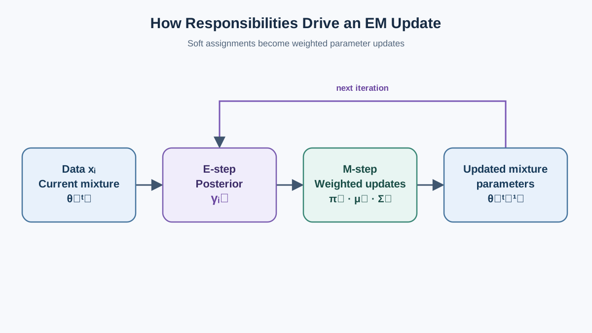
We cannot maximize the complete-data log-likelihood because it contains $z_{ik}$, which we never observe. So we replace each $z_{ik}$ with its expected value under the current parameters. That expectation is a posterior probability, and Bayes' rule gives it to us.

Apply Bayes' rule to $p(z_{ik} = 1 \mid x_i, \theta)$:

$$p(z_{ik} = 1 \mid x_i, \theta) = \frac{p(z_{ik} = 1) \, p(x_i \mid z_{ik} = 1, \theta)}{p(x_i \mid \theta)}$$

Expand the numerator into weight times density, and the denominator into the sum over all components:

$$\gamma_{ik} = \frac{\pi_k \, \mathcal{N}(x_i \mid \mu_k, \Sigma_k)}{\sum_{j=1}^{K} \pi_j \, \mathcal{N}(x_i \mid \mu_j, \Sigma_j)}$$

This $\gamma_{ik}$ is the responsibility: the posterior probability that point $i$ belongs to component $k$, given the data and the current parameters.

Three properties matter.

First, responsibilities across components sum to one for each point, because they are a probability distribution over $k$:

$$\sum_{k=1}^{K} \gamma_{ik} = 1$$

Second, they are a soft assignment. A point near a component's center gets a responsibility close to $1$ for that component. A point in the overlap region gets split responsibilities. When components are well separated, one responsibility dominates and the soft assignment collapses toward a hard one — which is why a converged mixture often looks like a clustering.

Third, this is where the soft-membership probabilities you have seen in a mixture model actually come from. They are not a heuristic. They are the exact posterior under the current parameters.

The M-Step: Maximizing Expected Complete Log-Likelihood

The E-step gave us responsibilities. The M-step asks: holding those responsibilities fixed, which parameters maximize the expected complete-data log-likelihood?

Define the Q-function as the expectation of the complete-data log-likelihood under the current responsibilities:

$$Q(\theta) = \sum_{i=1}^{N} \sum_{k=1}^{K} \gamma_{ik} \left[ \log \pi_k + \log \mathcal{N}(x_i \mid \mu_k, \Sigma_k) \right]$$

The responsibilities replaced the unknown $z_{ik}$. Now maximize $Q$ with respect to each parameter.

Weights

The weight terms are $\sum_i \sum_k \gamma_{ik} \log \pi_k$, subject to the constraint $\sum_k \pi_k = 1$. Handle the constraint with a Lagrange multiplier $\lambda$:

$$\frac{\partial}{\partial \pi_k} \left[ \sum_{i} \sum_{k} \gamma_{ik} \log \pi_k + \lambda \left( \sum_{k} \pi_k - 1 \right) \right] = 0$$

Differentiating gives $\frac{1}{\pi_k} \sum_i \gamma_{ik} + \lambda = 0$, so $\pi_k = -\frac{1}{\lambda} \sum_i \gamma_{ik}$. Summing over $k$ and using the constraint pins $\lambda = -N$, leaving:

$$\pi_k = \frac{1}{N} \sum_{i=1}^{N} \gamma_{ik}$$

The weight is the average responsibility for component $k$. Interpret $\sum_i \gamma_{ik}$ as the soft count of points assigned to component $k$; the weight is that count divided by $N$.

Means

Only the Gaussian term depends on $\mu_k$. Write out the log-density and keep the $\mu_k$-dependent part:

$$\log \mathcal{N}(x_i \mid \mu_k, \Sigma_k) = -\frac{1}{2}(x_i - \mu_k)^\top \Sigma_k^{-1} (x_i - \mu_k) + \text{const}$$

Differentiate $Q$ with respect to $\mu_k$ and set to zero:

$$\sum_{i} \gamma_{ik} \, \Sigma_k^{-1} (x_i - \mu_k) = 0$$

Since $\Sigma_k^{-1}$ is invertible, it drops out, and solving for $\mu_k$:

$$\mu_k = \frac{\sum_{i=1}^{N} \gamma_{ik} \, x_i}{\sum_{i=1}^{N} \gamma_{ik}}$$

The mean is a responsibility-weighted average of the data points. Each point pulls the mean toward itself in proportion to how much that component currently explains it.

Covariances

Differentiate $Q$ with respect to $\Sigma_k$. The result, after using the standard matrix derivative of the log-determinant and the quadratic form, is:

$$\Sigma_k = \frac{\sum_{i=1}^{N} \gamma_{ik} \, (x_i - \mu_k)(x_i - \mu_k)^\top}{\sum_{i=1}^{N} \gamma_{ik}}$$

This is a responsibility-weighted outer product of centered deviations — the soft analog of the sample covariance.

One detail deserves attention: the denominator. Dividing by $\sum_i \gamma_{ik}$ gives the maximum likelihood estimate, which is biased. Dividing by $N$ instead gives the maximum likelihood estimate for the mixture as a whole. Some implementations use a different denominator to reduce collapse. The choice is a bias-variance tradeoff, and it matters most when a component has few effective points.

The pattern across all three updates is the same: every parameter is a weighted statistic, and the responsibilities act as soft counts.

A Worked Two-Component Example by Hand

Numbers make the mechanism visible. Take four one-dimensional points: $x = \{1, 2, 4, 5\}$, and two components with fixed initial parameters:

Parameter	Component 1	Component 2
$\pi_k$	0.5	0.5
$\mu_k$	1.5	4.5
$\sigma_k^2$	1.0	1.0

E-step. For each point, compute the unnormalized responsibility $\pi_k \mathcal{N}(x_i \mid \mu_k, \sigma_k^2)$ and normalize. Using the Gaussian density with $\sigma^2 = 1$:

$x_i$	$\pi_1 \mathcal{N}(x_i \mid 1.5, 1)$	$\pi_2 \mathcal{N}(x_i \mid 4.5, 1)$	$\gamma_{i1}$	$\gamma_{i2}$
1	0.5 × 0.1295	0.5 × 0.0001	0.999	0.001
2	0.5 × 0.3521	0.5 × 0.0029	0.992	0.008
4	0.5 × 0.0029	0.5 × 0.3521	0.008	0.992
5	0.5 × 0.0001	0.5 × 0.1295	0.001	0.999

M-step. Now recompute the parameters using these responsibilities.

Soft counts: $N_1 = 0.999 + 0.992 + 0.008 + 0.001 = 2.0$, and $N_2 = 2.0$ by symmetry.

New weights: $\pi_1 = \pi_2 = 2.0 / 4 = 0.5$.

New mean for component 1:

$$\mu_1 = \frac{0.999(1) + 0.992(2) + 0.008(4) + 0.001(5)}{2.0} \approx \frac{3.020}{2.0} \approx 1.51$$

New variance for component 1:

$$\sigma_1^2 = \frac{0.999(1 - 1.51)^2 + 0.992(2 - 1.51)^2 + 0.008(4 - 1.51)^2 + 0.001(5 - 1.51)^2}{2.0} \approx 0.38$$

The component tightened around the points it already explained. Component 2 mirrors this around $4.5$.

Log-likelihood before and after. Before the update, the observed-data log-likelihood is $\sum_i \log(\pi_1 \mathcal{N}(x_i \mid 1.5, 1) + \pi_2 \mathcal{N}(x_i \mid 4.5, 1))$. After the update, recompute with the new parameters. The value rises. It always does — that is the next section.

Geometrically: the responsibilities pulled each mean toward the points it currently explains best, and the variance shrank because the component's effective points are now closer to its center. That is the whole algorithm in miniature.

Why the Likelihood Never Decreases

Monotone ascent is not a lucky property. It falls out of a decomposition.

For any distribution $q(Z)$ over the latent assignments, the observed-data log-likelihood decomposes as:

$$\ell(\theta) = \mathcal{L}(q, \theta) + \mathrm{KL}\!\left(q(Z) \,\|\, p(Z \mid X, \theta)\right)$$

where $\mathcal{L}(q, \theta)$ is a lower bound (the evidence lower bound, or ELBO) and the second term is a KL divergence between $q$ and the true posterior.

The KL divergence is always non-negative, so $\mathcal{L}(q, \theta) \le \ell(\theta)$. The bound touches the likelihood exactly when $q$ equals the posterior.

The E-step sets $q(Z)$ to the exact posterior $p(Z \mid X, \theta)$, which drives the KL term to zero. The bound rises to meet the likelihood — it becomes tight.

The M-step then maximizes $\mathcal{L}(q, \theta)$ with respect to $\theta$, holding $q$ fixed. Since the bound was already equal to the likelihood, raising the bound raises the likelihood.

So each full iteration cannot decrease $\ell(\theta)$. The sequence is monotone non-decreasing and bounded above, which guarantees convergence to a stationary point.

State the limit honestly: a stationary point is not the global maximum. The likelihood surface for a mixture has multiple local maxima, and EM will settle into whichever one its starting point leads toward.

Assumptions, Degeneracies, and Local Optima

The derivation quietly assumes several things. Each one has a failure mode.

Covariance degeneracy. Nothing in the updates prevents a component from collapsing onto a single data point. As $\sigma_k^2 \to 0$, the Gaussian density at that point diverges, and the likelihood goes to infinity. The M-step will happily walk into this singularity. In practice you regularize the covariance — add a small value to the diagonal, or impose a variance floor — to keep components from imploding.

Local optima and initialization. The likelihood has bad stationary points that can be arbitrarily worse than the global maximum. Different initial parameters reach different solutions. This is not a bug in the derivation; it is a property of the objective. Multiple restarts with different initializations are the standard mitigation.

Label switching. Component indices are not identified. Swapping the labels of components 1 and 2 produces an identical likelihood. Fitted parameters are only meaningful up to permutation, which matters when you try to compare runs or track a component across iterations.

Model misspecification. The derivation assumes Gaussian components and a fixed $K$. Neither is validated by the likelihood. A larger $K$ always fits at least as well, so the likelihood alone cannot choose the number of components.

From Derivation to Practice

The math predicts the operational decisions directly.

Because the likelihood has local optima, multiple restarts with sensible initialization matter. The derivation tells you why: the E-step's responsibilities depend entirely on where you start, and a bad start locks the algorithm into a poor basin. Initializing means from a quick K-means pass is a common and reasonable choice.

Because the likelihood increases monotonically with $K$, you cannot use it alone to choose the number of components. Information criteria that penalize complexity, or held-out likelihood, give you a defensible comparison. A component that shrinks to near-zero weight is a sign you asked for too many.

Because responsibilities are posterior probabilities, they carry uncertainty information. A point with $\gamma_{i1} = 0.51$ is genuinely ambiguous between two components. That is a signal, not noise — it tells you where the model cannot separate structure.

My rule for when this derivation is the right tool: use it when you need probabilistic assignments, when components have different shapes or orientations, or when the soft membership itself is the answer. Reach for something simpler when you only need hard groups and roughly spherical clusters — K-means is a special case of this model with fixed, equal, isotropic covariances, and it is faster.

The log-of-sum was never the real problem. The missing latent variable was. Once you see responsibilities as soft counts, every update is a weighted statistic, and the algorithm stops looking like magic.

Here is the next step I would take: fit a two-component mixture to a small dataset with scikit-learn, then compute the responsibilities by hand using the fitted weights, means, and covariances. If your hand-computed $\gamma_{ik}$ matches the library's predict_proba, you have understood the E-step. If it does not, the mismatch will tell you exactly which assumption you got wrong.