
Deriving Gradient Updates From a Differentiable Model Objective
You can write theta = theta - lr * grad from memory and still freeze when someone asks where grad came from. That gap is the whole problem. The update rule…

Key topics
You can write theta = theta - lr * grad from memory and still freeze when someone asks where grad came from. That gap is the whole problem. The update rule is not a magic spell you memorize. It is a short derivation you can rebuild from any differentiable objective.
This article is a derivation drill. We will pick a simple objective, differentiate it, read the update rule off the result, and then watch what the step size does to the path. By the end, you should be able to look at a new objective and derive its update yourself instead of hunting for a formula.
Why the Update Rule Looks Like Magic
Most beginners meet gradient descent in the same order: someone shows a loss function, someone shows an update rule, and the two are connected by a hand wave. You learn that the gradient points "downhill" and that you subtract it. You nod. You move on.
Then you hit a new objective — a weighted loss, a regularized model, a custom penalty — and you have no idea how to update anything. You can recite the rule but you cannot rebuild it.
The fix is to treat the update rule as a consequence, not a definition. Given an objective, the update falls out of a small amount of calculus. That is the durable skill. The specific optimizer you use later is replaceable; the derivation is not.
Before we start, let us be honest about the assumptions. We assume the objective is differentiable in the parameters — meaning we can compute its slope everywhere we care about. We assume we only use first-order information (the gradient, not curvature). And we assume we take small steps, because the math we use is only accurate locally. Hold onto that last one; it explains almost every training failure you will ever debug.
Notation Before Formulas
I want every symbol defined before it appears in an equation. Skipping this step is why derivations feel like fog.
- Parameters: the numbers the model learns. When there are many, we collect them into a vector (theta). For the worked example, we will use a single scalar parameter .
- Objective: a scalar function that measures how wrong the model is. Smaller is better. We want to minimize it.
- Gradient: the vector of partial derivatives, written . A partial derivative is a derivative where you hold every other variable constant and ask how the objective changes when only one parameter moves. The gradient stacks all those partials together.
- Step size (also called the learning rate): a small positive scalar, written (eta) or
lr, that controls how far we move along the descent direction. - Iteration index: , so is the parameter value at step .
One plain-language translation carries the whole idea: the gradient points in the direction of steepest increase, so its negative points in the direction of steepest decrease. Everything below is just making that sentence precise enough to compute with.
From Objective to Update: The Derivation
Start with the goal. We want the parameter value that minimizes :
We cannot solve this directly for most objectives, so we take an iterative approach. Suppose we are sitting at some current value . We want to choose a small change — call it — so that the new objective is smaller than .
To reason about small changes, we use a first-order Taylor expansion. This says that for a small step, the objective changes approximately by the gradient dotted with the step:
Read that second term carefully. It is the only part that depends on our choice of . To make the objective decrease, we need that term to be negative:
Now ask: what choice of makes this most negative? The dot product of two vectors is most negative when they point in opposite directions. So the best descent direction is the one directly opposed to the gradient:
We introduce the step size as the scalar that controls how far we move along that direction:
Substituting this back gives the update rule:
That is the whole derivation. Each piece has a job:
| Piece | What it does |
|---|---|
| Where we are now | |
| Which way is uphill | |
| The minus sign | Flip it to go downhill |
| How far to travel |
The descent condition is the fine print. This update is guaranteed to decrease only when the step is small enough that the Taylor approximation still holds. It is a local guarantee — it says nothing about whether you will reach the global minimum. That caveat is not pedantry. It is the reason step size matters so much.
Knowledge check
Check your understanding
Answer this question before you continue.
A Worked Example You Can Check by Hand
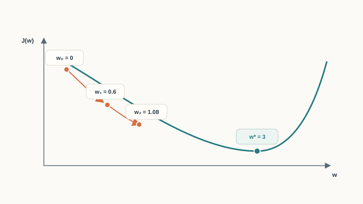
Let us make this concrete with an objective simple enough to differentiate in your head:
This is a parabola with its minimum at . The gradient is:
Start at with step size . Apply the update three times.
Iteration 1. Gradient is . Update: . Objective: .
Iteration 2. Gradient is . Update: . Objective: .
Iteration 3. Gradient is . Update: . Objective: .
| Iteration | Gradient | ||
|---|---|---|---|
| 0 | 0.000 | 9.00 | -6.00 |
| 1 | 0.600 | 5.76 | -4.80 |
| 2 | 1.080 | 3.69 | -3.84 |
| 3 | 1.464 | 2.36 | -3.07 |
Two things to notice. First, the parameter marches toward 3 and the objective falls every step. Second, the moves shrink. As approaches the minimum, the gradient approaches zero, so each update gets smaller. The geometry is exactly what the algebra promised: the gradient is the slope of the curve, and the update slides down that slope.
Knowledge check
Check your understanding
Answer this question before you continue.
What Step Size Actually Changes
Now rerun the same starting point, , with different step sizes. The objective has not changed. Only has.
For this particular objective, we can do better than guess. Define the distance from the minimum as . Substitute the update rule and simplify:
That single number, , is the error multiplier. It tells you everything about the path. If its absolute value is below 1, the distance shrinks and you converge. If it is negative, the sign flips each step and you oscillate. If its absolute value is at least 1, the distance does not shrink and you diverge.
| Step size | Error multiplier | Behavior |
|---|---|---|
| 0.01 | 0.98 | Slow, monotone approach |
| 0.1 | 0.80 | Fast, monotone approach |
| 0.5 | 0.00 | Lands exactly on the minimum in one step |
| 0.9 | -0.80 | Oscillates, but the distance still shrinks |
| 1.1 | -1.20 | Oscillates and grows — diverges |
Now the earlier list makes sense, and one entry changes meaning. With , the parameter does overshoot and the sign does flip each step — but the objective still falls every iteration, because the distance from the minimum shrinks by a factor of 0.8 each time. Overshooting is not the same as failing. Only when does the objective actually grow.
Common mistake: Beginners see a parameter jump past the minimum and assume training is broken. Watch the objective, not the parameter. Oscillation with a shrinking distance is still convergence.
Why does the general case need the small-step caveat if this example is exact? Because a parabola is a quadratic, and a first-order Taylor expansion of a quadratic is not an approximation at all — it is the function. For a curved, non-quadratic objective, the linear term only describes the surface near your current point. Step too far and you leave the neighborhood where that description holds, so the "descent direction" stops being a descent direction. The parabola gives you an exact, checkable model of the mechanism; real objectives give you the local version.
Common mistake: When loss jumps up or oscillates, beginners blame the model, the data, or the features. Check the step size first. A learning rate that is too high produces exactly this signature, and it is the cheapest thing to fix.
Knowledge check
Check your understanding
Answer this question before you continue.
When This Derivation Applies — and When It Breaks
The derivation rests on a few conditions. Know them so you can tell when the update rule is the wrong tool.
It applies when the objective is differentiable in the parameters and you can compute or reasonably approximate the gradient. That covers a large share of classical models: linear regression with squared error, logistic regression with cross-entropy, and many regularized variants.
It weakens or breaks when:
- The objective is non-differentiable (for example, a hard count or a step function), so no gradient exists.
- Gradients are noisy or vanishing, so the direction you compute is unreliable.
- Features are badly scaled. Scaling changes the shape of the objective — it stretches the parabola into a narrow valley — which changes the effective step size in each direction. This is why feature scaling shows up again and again in practical training.
More advanced optimizers exist, and they are worth learning later. But they all rest on the same idea you just derived: compute a gradient, take a step against it. The derivation is the foundation; the optimizer is the variation.
Knowledge check
Check your understanding
Answer this question before you continue.
Verify the Derivation in a Few Lines of NumPy
The code here is a check on the math, not a new lesson. It should reproduce the table above.
import numpy as np

def J(w):
    return (w - 3.0) ** 2

def grad_J(w):
    return 2.0 * (w - 3.0)

w = 0.0
lr = 0.1
for t in range(4):
    print(f"t={t}  w={w:.3f}  J(w)={J(w):.3f}  grad={grad_J(w):.3f}")
    w = w - lr * grad_J(w)
If the printed values match the hand-computed table, your derivation is correct. As a second check, compare the analytic gradient to a finite-difference estimate:
eps = 1e-6
w_test = 1.0
numeric = (J(w_test + eps) - J(w_test - eps)) / (2 * eps)
print(numeric, grad_J(w_test))  # should agree closely
When the analytic and numeric gradients agree, you have confirmed the derivative. When they disagree, you have a bug in your math, not in your optimizer.
The Rule to Carry Forward
Before you trust any training run, do two things. First, derive the update from the objective so you know what the code is actually doing. Second, watch whether the loss falls — if it rises or oscillates, suspect the step size before anything else.
The derivation is the durable skill. The specific optimizer is replaceable. Your next step is to apply this same process to a real model objective: take the least-squares loss for a linear model, differentiate it with respect to each coefficient, and read off the update rule. Same drill, more parameters, and now you know exactly where the minus sign comes from.
Knowledge check
Final check
Finish the article by checking the ideas you just learned.
References
Build stronger machine learning foundations
Use structured resources to connect theory, scikit-learn workflows, and evaluation practice.


