
Missing Data in Machine Learning: When Imputation Helps or Lies
Every beginner hits the same wall: you load a real dataset, and it is full of holes. Columns you need are dotted with NaN. Your model refuses to run. So…

Key topics
Every beginner hits the same wall: you load a real dataset, and it is full of holes. Columns you need are dotted with NaN. Your model refuses to run. So you reach for the two reflexes everyone teaches: drop the rows with dropna(), or fill the blanks with the column mean.
Both reflexes are half right. Dropping rows is sometimes the correct call. Mean imputation is a fine baseline. But here is what the reflex hides: filling a blank is not recovering truth. It is manufacturing an estimate and then asking your model to trust it as if it were a real measurement.
The real question is not "how do I fill the blanks?" It is "what is the missingness telling me, and where does the fill belong in my workflow?" Once you can answer those two questions, you can choose a defensible missing-value strategy instead of guessing.
Why Your First Instinct About Missing Values Is Half Right
Let's give the reflex its due. Mean imputation is cheap, fast, and it keeps your dataset intact. Dropping rows is even simpler. When missing values are rare and random, both approaches work fine.
The problem is that they stop working the moment missingness has a pattern. And in real data, missingness usually has a pattern.
Here is the mechanism to understand: statistical learning procedures do not care much about the mean of a feature. They care about the relationship between the variance of one feature and the variance of another. When you replace missing values with a single constant like the mean, you collapse that variance structure. Every imputed row now has an identical value for that column, which quietly distorts the relationships your model is trying to learn.
Think of it this way. A mean fill does not add information. It adds a placeholder that pretends to be information. The model cannot tell the difference between a real measurement and your placeholder, so it treats both with the same confidence.
That is why the reason for missingness matters more than the fill method. Before you choose a strategy, you need to know why the data is missing in the first place.
Three Reasons Values Go Missing (and Why the Reason Matters)
Statisticians classify missingness into three mechanisms. The names sound academic, but each one changes what you can safely do with your data.
Missing completely at random (MCAR). The blank is unrelated to any value, observed or unobserved. Imagine a sensor that randomly drops a reading now and then, with no pattern to which readings get lost. The rows with missing values are just a random sample of your full dataset. This is the friendliest case: dropping rows or using simple imputation is least risky here.
Missing at random (MAR). The blank depends on observed features, but not on the missing value itself. Suppose you run a survey and older customers are less likely to report their income. Age is observed, income is missing, and the missingness tracks age. If you know someone's age, you have a decent clue about whether their income field will be blank. This is more common than MCAR, and it means you can often predict missingness from the data you already have.
Missing not at random (MNAR). The reason for the blank is tied to the value that is missing. High earners refuse to report their income. Patients skip a question about a sensitive symptom. The very fact that the value is absent tells you something about what the value would have been. This is the dangerous case. Imputation can actively mislead you here, because the blank itself carries signal that a naive fill will bury.
Here is a small table showing the same feature under each mechanism:
| Mechanism | Why the value is missing | What a naive fill hides |
|---|---|---|
| MCAR | Random equipment or recording failure | Nothing much; the fill is a harmless estimate |
| MAR | Depends on another observed feature | The relationship between missingness and that feature |
| MNAR | Depends on the missing value itself | The fact that absence is informative |
The uncomfortable truth: in practice, you rarely know the mechanism with certainty. You can inspect patterns and make educated guesses, but you cannot prove why a value is absent. So you plan defensively. You assume missingness might be informative, and you build your strategy so that a wrong guess does not silently corrupt your model.
Knowledge check
Check your understanding
Answer this question before you continue.
The Imputation Toolbox: Simple Fills, Neighbor Fills, Model Fills
Once you have a sense of why values are missing, you can choose a fill method. The options range from simple to sophisticated, and each one carries assumptions.
Constant and statistic fills. Mean, median, and most-frequent imputation replace blanks with a single computed value. These are cheap and reasonable baselines. But they collapse variance, as we discussed, and they ignore relationships between features. If income is missing more often for older customers, a mean fill will not capture that pattern.
Missingness indicators. This is the quiet workhorse of imputation. Instead of only filling the blank, you add a column that flags whether the original value was missing. In scikit-learn, the add_indicator option on imputers does exactly this. The indicator column lets your model use "this value was absent" as a feature in its own right. Even when your fill is crude, the indicator preserves the signal that missingness itself might carry.
KNN and iterative imputation. These methods use relationships in the data to estimate blanks. KNN imputation finds similar rows and borrows their values. Iterative imputation models each feature as a function of the others and fills values round by round. Both are more expressive than a mean fill, and both are more expensive. They are still estimates. A sophisticated guess is still a guess.
Here is the practical guidance from scikit-learn's own documentation, and I think it is worth taking seriously: for prediction, a simple imputer plus an expressive downstream model often matches sophisticated imputation. Fancy imputation earns its cost mainly when reconstructing the data itself is the goal, not when you are trying to predict an outcome.
So the toolbox is not a ladder you must climb. Start simple. Add an indicator. Let your model do the heavy lifting.
Knowledge check
Check your understanding
Answer this question before you continue.
When Missingness Itself Is the Signal
Here is where the reflex gets expensive. A blank is not always noise to erase. Sometimes the very fact that a value is absent predicts the outcome.
Consider a form field that only certain users skip. Maybe the field asks about a topic that correlates with the target you are trying to predict. If the act of skipping correlates with the outcome, then dropping the row throws away the example entirely, and filling the blank buries the signal under a fake value.
The fix is the missingness indicator. By adding a column that records whether the value was present, you give the model permission to learn "this value was absent" as a feature. The fill becomes a placeholder for the algorithms that need complete data, and the indicator carries the real information.
Here is the decision rule I use: if you suspect the blank itself predicts the outcome, keep an indicator alongside whatever fill you choose. The indicator is cheap, it preserves information, and it protects you when your guess about the missingness mechanism is wrong.
Knowledge check
Check your understanding
Answer this question before you continue.
The Leakage Trap: Why Imputation Must Live Inside the Pipeline
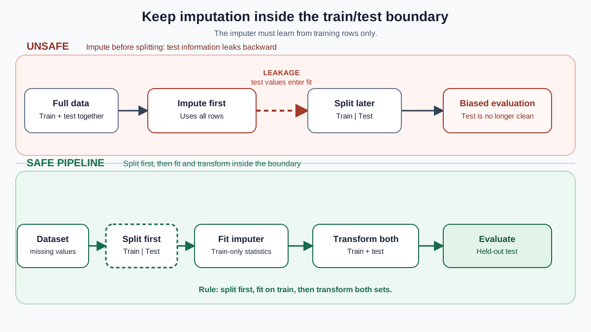
Now the mistake that quietly corrupts more beginner projects than any other: computing imputation statistics on the full dataset before splitting.
Here is the classic error. You load your data, compute the mean of a column, fill the blanks, and only then split into training and test sets. It feels harmless. The mean is just a number, right?
Wrong. That mean was computed using test rows. Information from the test set has crossed the evaluation boundary and leaked into your training data. Your model will look better in evaluation than it will in the real world, because it had a peek at the future during training.
The fix is conceptually simple: fit the imputer on the training split only, then transform the test split with those same learned values. The imputer learns its statistics from training rows, and test rows are transformed using statistics they did not help create.
This is exactly what a scikit-learn pipeline enforces. When you bundle your imputer into a pipeline, the fit happens on training data and the transform applies to both splits without leakage. This is a strong reason to keep imputation inside a pipeline rather than doing it as a standalone pandas step before you split.
Common mistake: Computing
df.fillna(df.mean())before splitting your data. Every statistic computed before the split is information from the future crossing into your training set. Fit the imputer on training data only.
Knowledge check
Check your understanding
Answer this question before you continue.
Choosing a Strategy: A Decision Rule for Beginners
When you sit down with a messy dataset, work through this decision flow:
First, inspect how much is missing and why. Look at each column with blanks. What fraction of rows is affected? Is there a pattern to which rows are missing? Do you have domain knowledge about why the data was not collected?
Then choose among four options:
Drop the rows. Fine when missingness is rare and you have reason to believe it is MCAR. Risky when blanks are common or meaningful, because you shrink your sample and can bias the model. If 30 percent of your rows have a missing value in one column, dropping them all is throwing away nearly a third of your data.
Drop the feature. Reasonable when a column is mostly empty and carries little signal. If 90 percent of a column is missing, that column has very little information to offer. But this is wasteful when the column matters. A column can be 40 percent missing and still be the strongest predictor in your dataset.
Simple imputation plus an indicator. This is the pragmatic default for prediction. Fill with the median or mean, add a missingness indicator, and let your model sort out whether absence means something. It is cheap, it is leakage-safe inside a pipeline, and it preserves the option for the model to learn from missingness.
Sophisticated imputation. Worth considering when you have strong relationships between features and the missingness is MAR. But remember: for prediction, the gain over simple imputation is often marginal. Invest here mainly when reconstructing the data itself is the goal.
Here is the honest caveat that should shape your whole approach: every imputed value is an estimate. You are not recovering data that was never collected. You are manufacturing a plausible placeholder and making its limitations visible through indicators and honest evaluation.
The goal is not a perfect reconstruction. The goal is a defensible workflow — one where you can explain why you chose each strategy, where the imputation lives on the right side of the train/test boundary, and where the model's evaluation scores reflect how it will actually perform on new data.
Your Next Step
Open your own dataset and inspect it with fresh eyes. For each column with missing values, ask three questions: How much is missing? Is there a pattern to which rows are missing? Does the absence itself seem informative?
Then commit to one change: place your imputation inside a pipeline so the split boundary stays clean. Let the imputer fit on training data only, and let the pipeline handle the rest.
The rows you drop and the values you fill are decisions, not chores. Make them deliberately, make their limits visible, and your model will reward you with evaluation scores you can actually trust.
Knowledge check
Final check
Finish the article by checking the ideas you just learned.
References
Research updated Sep 8, 2026


